
Research article · 2021 · Full text
International Journal of Biology SciencesThe assessment of floral abundance and composition of Neni-Nimo watershed in Anaocha L.G.A. of Anambra state, Nigeria
Volume 3(1) · Pages 01–09 · DOI: 10.33545/26649926.2021.v3.i1a.20 ↗
Research areasAfrican Botany and Ecology Studies
Abstract
Author-writtenThe research was carried out on the floral composition of Neni-Nimo watershed between November 2019 and July 2020. The research work aimed to find out the various plant species that inhabit the watershed, their abundance measures and importance values. In this study, the watershed was divided into three catchment areas, the upper, the middle and the lower catchment. Each of the catchment zones was divided into component parts, with an area of (50 m X 30 m) each. The experiment was laid in a randomized complete block design. A plotless sample technique called the centre point technique was used to ascertain importance values Indices (IVI) for trees, while the plot count sampling technique (quadrant) was employed for shrubs, forbs, grasses and climbers. Random sampling techniques were employed in all cases to eliminate bias. The encountered growth forms such as trees, shrubs, forbs, climbers and grasses were identified and recorded. The important values index (IVI) was obtained for all the growth forms. The encountered species were quantitatively analyzed for density, frequency and abundance or dominance depending on their various growth forms. The importance value indices for each of the species were determined by summing up relative density, relative frequency and relative abundance of the species. The result shows that trees were the most abundant flora in the upper catchment area with Elaeis guinensis being the most dominant species. At the middle catchment, shrubs were the most abundant flora, with Chromolaena odorata being the most dominant species. Also at the lower catchment area, shrubs were the most abundant flora, followed by grasses. Venonia amygdalina had the highest abundance for shrubs while Zea mays had the most abundance value for grasses at the lower catchment. The study revealed that most of the dominant species in the three catchment areas were crops of economic value which are planted by man.
Summary
Source-checkedPlain-language reading of the full paper, prepared with AI and checked against the text. Each point links to the authors' own words.
Why it matters
- Watersheds are land areas that collect precipitation runoff and drain water, nutrients, and sediments into nearby streams or water bodies. View evidence ↗
- Human activities, including agriculture and deforestation, impact watershed ecosystems and contribute to nutrient enrichment in water bodies. View evidence ↗
- Understanding the species composition of watersheds is critical for promoting the conservation of biological diversity. View evidence ↗
The question
- The study aimed to identify the plant species inhabiting the Neni-Nimo watershed and determine their abundance and importance values. View evidence ↗
What they did
- The research was conducted at the Ogbujilekwe stream watershed in Anambra State, Nigeria. View evidence ↗
- The watershed was divided into upper, middle, and lower catchment areas, each containing three replicates of 50m x 30m. View evidence ↗
- Trees were sampled using a point-centered plotless count technique, while shrubs, forbs, climbers, and grasses were sampled using quadrant plot counts. View evidence ↗
- The Importance Value Index (IVI) was calculated by summing relative density, relative frequency, and relative dominance (or abundance for non-forested areas). View evidence ↗
What they found
- The study identified 149 plant species from 45 families, including 40 trees, 30 shrubs, 39 forbs, and 27 grasses. View evidence ↗
- Among the 40 tree species, Elaeis guinensis was the most dominant with a dominance value of 120 and the highest IVI of 30.3, while Vocanga africana had the lowest dominance value of 2. View evidence ↗
- Vernonia amygdalina was the most abundant shrub, with an abundance value of 94.6% and an IVI of 130.9. View evidence ↗
- For grass species, Zea mays had the highest abundance (58.3) and IVI (52.8), whereas Setaria barbata had the lowest abundance (3.5) and IVI (3.9). View evidence ↗
- Flora abundance varied by zone: trees (dominated by Elaeis guinensis) were most abundant in the upper catchment, while shrubs (dominated by Chromolaena odorata) were most abundant in the middle and lower catchments. View evidence ↗
- While all growth forms were present in the upper and middle catchments, trees were completely absent in the lower catchment (current usage area). View evidence ↗
What it means
- The authors conclude that human influence has drastically reduced the natural plant composition of the watershed, leaving economic crops as the most dominant species. View evidence ↗
Visual summary
3 visualsIllustrations explain the paper; charts are replotted from the paper's own table values.
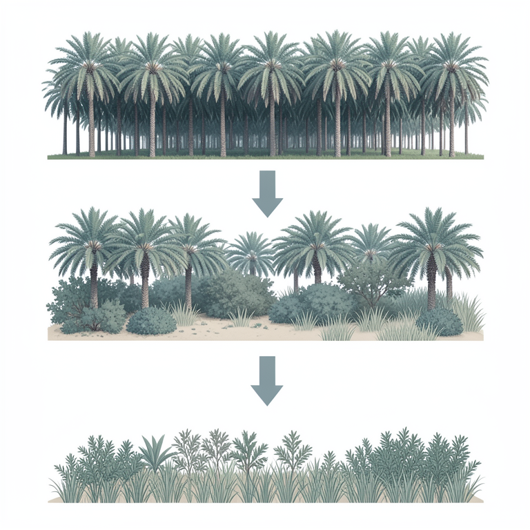
Zonal Floral Distribution
AI-generated conceptual illustration (A tropical watershed landscape in Nigeria featuring oil palms (Elaeis guinensis), shrubs (Chromolaena odorata), and wild). It explains the idea and does not show study data.
View source evidence ↗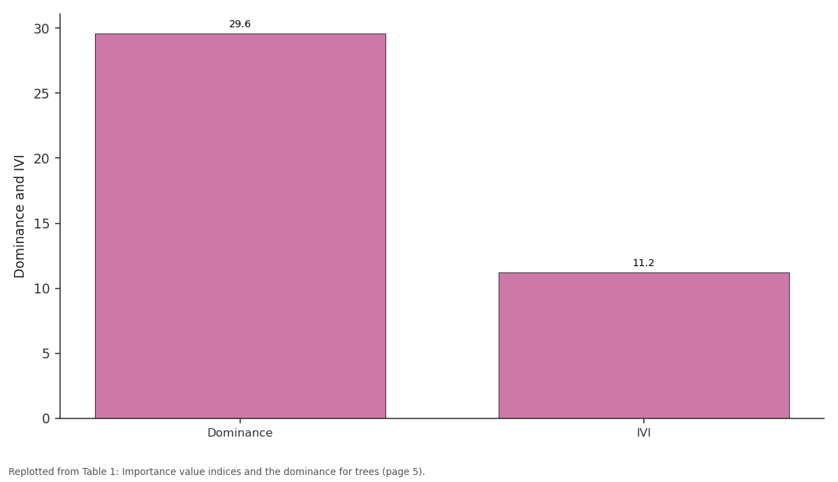
Diallum guineensis: Dominance vs IVI
Replotted from Table 1 (page 5) of the original paper. Every bar is the paper's own table value.
View source evidence ↗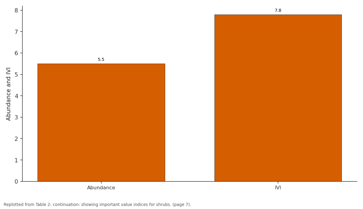
Uvaria chamae: Abundance vs IVI
Replotted from Table 2 (page 7) of the original paper. Every bar is the paper's own table value.
View source evidence ↗Figures & tables
From the original paper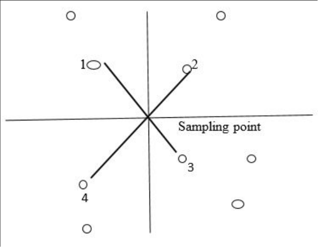 Figure 1
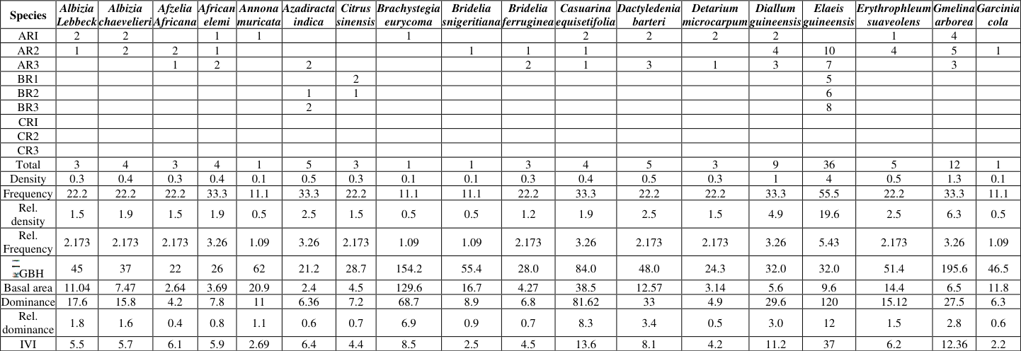 Table 1
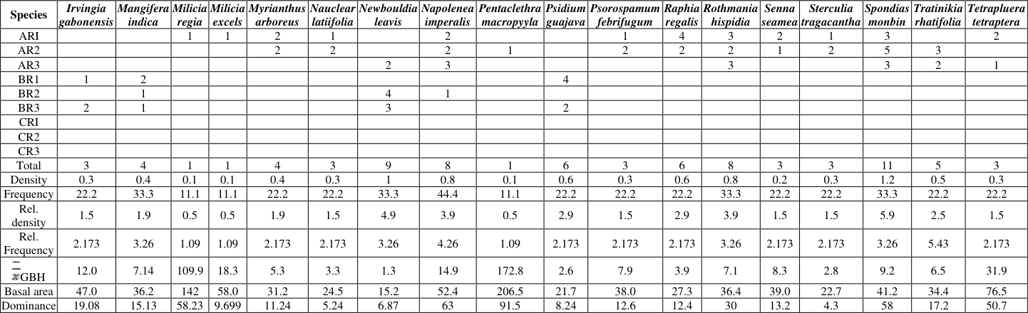 Table 1
 Table 1
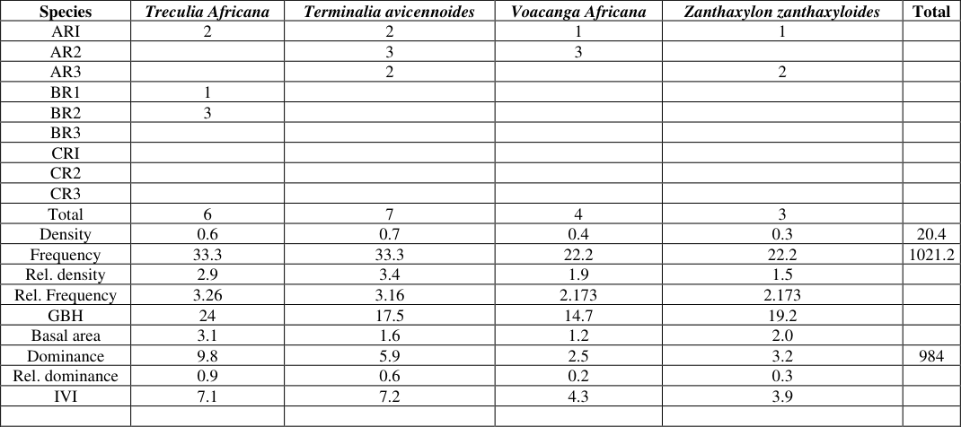 Table 1
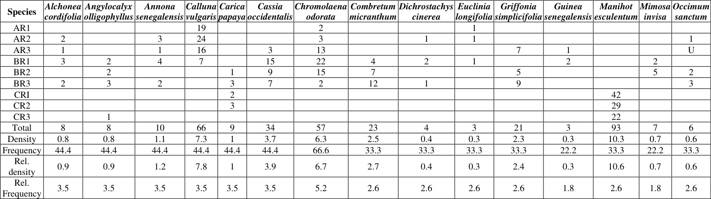 Table 2
 Table 2
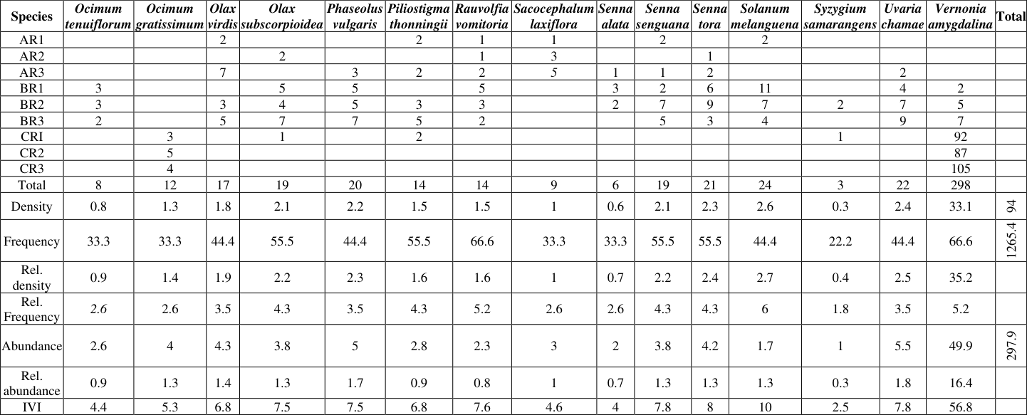 Table 2
 Table 3
 Table 3
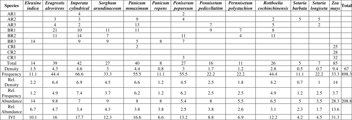 Table 3
Introduction
A watershed is a topographically delineated area that is bounded by a drainage divide, which collects run-off from precipitation and primarily drains large amounts of underground water, melted ice, nutrients, sediments and toxins, from the soil into the nearby water bodies or stream channels. The term watershed is synonymously used with a drainage basin although they are different (Enwelu et al., 2014) [6] . Watershed is made up of a riparian area or riparian zone which is the strip of vegetation along a stream with distinct composition and density from the surrounding upland. Because of its topographic nature, it drains underground water and nutrients into nearby streams from the predominant landscape surface types (Kunstler et al., 2004) [10] . The impacts of anthropogenic activities and nutrient fluxes from watersheds are dynamic over time and space. Nutrients from watersheds will result in to increase in nutrient in the nearby or receiving water (Howarth et al., 2012; Boyer et al., 2002.) [9, 3] . This nutrient enrichment vary to time and space, depending on many social, regulatory, economic and environmental drivers (Boyer et [3,14,8] and also determines the type of flora in that watershed. Most watersheds are usually thick and evergreen forest habitat, with varieties of flora and fauna composition. The activities of man have led to alterations of the environment which are both passive and diverse. These alterations range from altered atmospheric chemistry to dramatic modifications of the landscape for agricultural and urban uses (Vitousek et al., 1997; Kareiver et al., 2007 [15] . Increasingly, it has been recognized that human actions on watersheds such as deforestation and agricultural activities have created impacts on the ecosystem and is highly connected to the enrichment of nutrient in water bodies (Foley, 2005) [7] . Assessment of species composition entails studies of different plant life as they are naturally distributed on the watershed and their importance value. Importance value is the measure of how dominant a species is in a given forest area. It is usually calculated by summing up the relative frequency, relative density and relative dominance for trees and relative frequency, relative density and relative abundance for shrubs, DOI: https://doi.org/10.33545/26649926.2021.v3.i1a.20 forbs and grasses. Bhadra and Pattanayak (2017) [2] opined that dominance is justified for tree community as the individuals of tree species are available in higher girth and abundance is justified for shrubs, forbs and trees. Therefore important value index of species belonging to a tree and other communities should be evaluated based on dominance and abundance separately. Abundance and dominance are two aspects of plant species dynamic, often considered interchangeably together with frequency and density to estimate important value index (IVI) Importance value (IVI). Studies and knowledge of the specie composition of any area especially watersheds are important as it helps to encourage conservation of species. Conservation of biological diversity is essential for the survival of the human race, because it provides a livelihood for man and livestock, mitigate climatic changes and maintain samples of unchanged biotic communities in their natural form for breeding. Therefore, this research work aimed to find out the various plant species that inhabit the watershed, their abundance measures and importance values.
Materials and Method Experimental site
The study on species compositions was carried out at Ogbujilekwe stream watershed bordering Neni and Nimo town in Anaocha L.G. A. of Anambra State, Nigeria. The Ogbujilekwe stream, as explained by the villagers and some of the farmers in the area, cuts across four major towns in Anambra State namely; Neni, Nimo, Oraukwu and Adazi-Nnukwu. The Neni-Nimo watershed falls within the humid tropical climate belt of Nigeria. The two seasons experienced in this area are the rainy season and dry season. The maximum average rainfall is experienced during July and August. The mean annual rainfall is about 1500 -2500nm.
Experimental Design
The experiment was laid in a randomized complete block design (RCBD). The watershed was divided into three catchment areas, the upper, middle, and lower catchment, each of the catchments, had three replicates with an equal area of 50m x 30m. The catchments were demarcated from each other, using pegs.
Sampling procedure
A quantitative relationship between area and number of species was first developed by Arrhenius (1921) [1] , a pioneer in the area of Geographical ecology. Point centred plotless count technique was used for the sampling trees, while the plot count technique using quadrants were used for the forbs, shrubs, climbers and grasses. The species encountered were identified using Geogle lens applicaion, relevant texts like Handbook of West African Weed (Akobundu and Agyakwa, 1998). The vegetation data collected were quantitatively analyzed for density, frequency, relative density, relative frequency and basal area as per (Mishra, 1968) [11] . The importance value index (IVI) for each species was determined as the sum of relative density, relative frequency and relative dominance for the forested area or relative abundance for the non-forested areas (Phillips, 1959).
Survey Procedure for Trees
Survey Procedure for Trees
Details of Standard Procedure
The plotless sampling procedure was used for data collection for all trees. Four quarters were established at the sampling point using a cross made by two wooden frames. Firstly, the distance of the closest tree to the sampling point from four quadrants were measured. The averages of the four distances were calculated to obtain the mean distance occupied by trees. Finally, any tree whose stem was up to 4.3ft height had the girth measured immediately at this mark. The reliability of this method has been given by Cottan and Curtix (1994).
Okereke et al. (2016) [12] noted that one of the limitations of this method for field application is that an individual must be located within each quarter and an individual must not be measured twice. The diameter of a tree at 4.3 foot level is called diameter breast height (DBH). The basal area of the trees were calculated using the formulae BA= 0.005454× DBH^2 and it was used to ascertain the basal area of the plants. The number 0.005454 is called foresters constant and it comes by dividing π by 4×144. The number of individuals of each species were added up and used to estimate species composition and diversity. Bar charts were used to record species composition according to growth forms (tree, climbers, shrubs, grasses and forbs
Details of Standard Procedure for Shrubs, Forbs and Climbers
The plot count technique was achieved using the quadrant. The Plot count quadrant techniques are used in herbaceous sites with known boundaries and lacking physical obstacles. At first, the total length and width are obtained. The plots were then demarcated from each other using pegs and the size was ascertained. Then the sampling intensity was worked out by determining 5 % of the total plot size since ecology accepts of 5 % or 10 % for expediency. The sampling unit is a quadrant. Having known the sampling intensity, the number of quadrants to be placed in each of the plots was calculated by dividing sampling intensity by the size of the quadrant. The quadrant size in all cases is 2×1m in size.
Next is to determine the sampling points on the plot. This was achieved by using the random number technique. In this case, a set of random numbers were written according to the number of throws of the quadrant which is 38 the numbers were randomly picked before the experiment and the point of intersection of the numbers were marked with pegs. Density is defined as the number of individuals of particular species per unit area. It also gives an idea of how closely packed trees are growing in an area. Frequency is defined as the distribution or relative representation of a particular species or how species are spread out in a given area. Dominance is defined as the measure of the size or weight of vegetation. Abundance is defined as the number of individual species found in a particular sample. Basal area is defined as the sum of the cross sectional area of all the trees of a particular species measured at 4.3 ft above the ground. DBH is diameter at breast height of a tree species at 4.3 ft, and 0.005454 is known as foresters constant.
The formulae for calculating the important value indices (IVI) for trees is as follows
The formulae for calculating the important value indices (IVI) for trees is as follows
Result and Discussion
Result and Discussion
Species composition of the studied Watershed
The specie composition of the plants encountered in the three catchment zones was evaluated. A total of 149 plant species comprising of 40 trees, 30 shrubs, 39 forbs, 27 grasses and 13 forbs were encountered. The plant species encountered make up to 45 families. All the growth forms which include trees, forbs, shrubs, climbers and grasses were present in the upper catchment areas or forested area, and middle catchment or fallow areas, but in the lower catchment or current usage area, trees were totally absent.
Looking at Table 1 below, Out of the 40 trees encountered in the watershed, Elias guinensis, had the highest dominance value of 120 while Vocanga africana had the least dominance value of 2, Elias guinensis also had the highest importance value indices of 30.3 among the plant species while Garcinia cola has the least importance value indices (IVI). From Table 2 below, shrubs were mostly found in the fallow areas, followed by forested areas and very few were found in the current usage farm site. Vernonia amygdalina had the highest abundance value of 94.6% and very high important value indices (IVI) of 130.9, followed by Manihot escculenta with abundance value of 31% and important value indices of 17%. Syzygium samarangens had the least dominace value of 1% and important value indices (IVI) of 2.3. The abundance value for forb species showed that Ipomea aquarica scored the highest abundance value of 22.2, while Boreria verticulata had the least abundance value of 2.5. The evaluation of the importance value indices (IVI) also shows that Ipomea aquatica scored the highest importance value indices (IVI) of 19.1, Followed by Ageratum conyzoides with the IVI of 15.2 while Bryophyllum pinnatum had scored the least (IVI). Result from the climbers showed that Telfaria occidental followed by Peuraria phaseoloides scored the highest abundance of while Cissus araloides and T.occidentalis, had the highest importance value indices (IVI) of 35 and 33.5. Also Cucurbita pepo score the least abundance value of 3.5 and the least IVI value of 13.1. Table 3 shows the result for the grass species. Z. mays scored the highest abundance and IVI of 58.3 and 52.8 respectively while Seteria babarta had the least abundance and (IVI) of 3.5 and 3.9. Also from the graphical analysis showing the IVI of the grass species as presented in Figure 4.5a and b. Zea mays was also found to have the highest importance value index. In the study, the assessment of specie composition of Neni-Nimo degraded watershed, it was discovered that trees were the most dominant in the upper catchment area, and the most frequent tree species is Elaeis guinensis, (55%) however, the most dominant tree species also was Elaeis guinensis. For the shrubs, Vernonia amygdalina was the most abundant and the most dominant specie, with IVI of 56.8. At the middle catchment, shrubs were the most abundant with the most dominant specie being Chromolaena odorata, with abundance of 9.5 and Importance value indices IVI of 15.1. Also at the lower catchment area, shrubs were the most abundant, followed by grasses, Vernonia amagdalaena had the highest abundance of 49.9 for shrubs, followed by Zea mays, with abundance of 28.3 for grasses. The study revealed that most of the dominant species in the three catchment areas were mostly economic crops which are planted by man.
| Species | Eleusine indica | Eragrostis alrovirens | Imperata cylindrical | Sorghum arundinaceum | Panicum mmaximum | Panicum repens | Peniserum pepureum | Pennisetum pediccllatitm | Pernnisetum polystachion | Rottboelia cochinchinensis | Setaria barbata | Setaria longiseta | Zea mays | Total |
|---|---|---|---|---|---|---|---|---|---|---|---|---|---|---|
| AR1 | 4 | 2 | ||||||||||||
| AR2 | 3 | 3 | 9 | 4 | 2 | 5 | 5 | |||||||
| AR3 | 4 | 2 | 13 | 7 | 5 | 2 | ||||||||
| BR1 | 21 | 10 | 11 | 11 | 9 | 7 | 8 | |||||||
| BR2 | 11 | 14 | 7 | 11 | 4 | 11 | ||||||||
| BR3 | 14 | 9 | 9 | 5 | 8 | 7 | ||||||||
| CRI | 2 | 25 | ||||||||||||
| CR2 | 28 | |||||||||||||
| CR3 | 3 | 32 | ||||||||||||
| Total | 14 | 39 | 42 | 27 | 40 | 8 | 27 | 16 | 11 | 26 | 5 | 7 | 85 | |
| Density | 1.5 | 4.3 | 4.6 | 3 | 4.4 | 0.8 | 3 | 1.7 | 1.2 | 2.8 | 0.5 | 0.7 | 9.4 | 67 |
| Frequency | 11.1 | 44.4 | 66.6 | 33.3 | 55.5 | 11.1 | 55.5 | 22.2 | 22.2 | 44.4 | 11.1 | 22.2 | 33.3 | 898.3 |
| Rel. Density | 2.2 | 6.4 | 6.9 | 4.5 | 6.6 | 1.2 | 4.5 | 2.5 | 1.8 | 4.2 | 0.7 | 1 | 14 | |
| Rel. Frequency | 1.2 | 4.9 | 7.4 | 3.7 | 6.2 | 1.2 | 6.2 | 2.5 | 2.5 | 4.9 | 1.2 | 2.5 | 3.7 | |
| Abundance | 14 | 9.8 | 7 | 9 | 8 | 8 | 5.4 | 8 | 5.5 | 6.5 | 5 | 3.5 | 28.3 | 208.8 |
| Rel. Abundance | 6.7 | 4.7 | 3.4 | 4.3 | 3.8 | 3.8 | 2.5 | 3.8 | 2.6 | 3.1 | 2.3 | 1.7 | 13.6 | |
| IVI | 10.1 | 16 | 17.7 | 12.3 | 16.6 | 6.6 | 13.2 | 8.8 | 6.9 | 12.2 | 4.2 | 4.5 | 31.3 |
Table text extracted from the original PDF; superscript letters are shown inline. The original table image is below.
View original table image
| Density | 3.4 | 5.5 | 0.7 | 1.2 | 2.8 | 0.7 | 1.2 | 0.9 | 0.6 | 2.2 | 2.7 | 4.8 | 1.8 | 1.5 |
|---|---|---|---|---|---|---|---|---|---|---|---|---|---|---|
| Frequency | 33.3 | 55.5 | 22.2 | 22.2 | 44.4 | 22.2 | 33.3 | 22.2 | 22.2 | 44.4 | 44.4 | 44.4 | 22.2 | 33.3 |
| Rel. Density | 5 | 8.2 | 1 | 1.8 | 4.2 | 1 | 1.8 | 1.3 | 0.9 | 3.3 | 4 | 7.2 | 2.7 | 2.2 |
| Rel. Frequency | 3.7 | 6.2 | 2.5 | 2.5 | 4.9 | 2.5 | 3.7 | 2.5 | 2.5 | 4.9 | 4.9 | 4.9 | 2.7 | 3.7 |
| Abundance | 10.3 | 10 | 3.5 | 5.5 | 8 | 3.5 | 6.7 | 4.5 | 3 | 6.3 | 6.3 | 11 | 8.5 | 4.7 |
| Rel. Abundance | 4.9 | 4.8 | 1.7 | 2.6 | 3.8 | 1.7 | 3.2 | 2.2 | 1.4 | 3 | 3 | 5.2 | 4 | 2.3 |
| IVI | 13.6 | 19.2 | 5.2 | 6.9 | 12.9 | 5.2 | 8.7 | 6 | 8 | 11.2 | 11.9 | 17.3 | 9.4 | 8.2 |
Table text extracted from the original PDF; superscript letters are shown inline. The original table image is below.
View original table image
| Species | Acroceras zizanioides | Andropogon gayanus | Andropogon tectorum | Axonopus compressus | Bambusa vulgaris | Brachiara deflexa | Brachiaria ruziziensis | Chloris pilosa | Cynopogon cittratus | Cynodon dactylon | Hackelochloa granularis | Digitaria horizontalis | Digitaria nuda | Echinochloa obtusiflora |
|---|---|---|---|---|---|---|---|---|---|---|---|---|---|---|
| AR1 | 7 | 4 | 7 | |||||||||||
| AR2 | 5 | 2 | 5 | 5 | 3 | 4 | 4 | |||||||
| AR3 | 5 | 5 | 2 | 3 | 4 | |||||||||
| BR1 | 11 | 11 | 11 | 5 | 4 | 7 | 5 | 20 | 2 | |||||
| BR2 | 7 | 2 | 2 | 7 | 13 | 7 | 5 | |||||||
| BR3 | 10 | 13 | 7 | 11 | 9 | 7 | 10 | |||||||
| CRI | 4 | 4 | 3 | |||||||||||
| CR2 | 2 | 2 | ||||||||||||
| CR3 | ||||||||||||||
| Total | 31 | 50 | 7 | 11 | 26 | 7 | 11 | 9 | 6 | 20 | 25 | 44 | 17 | 14 |
Table text extracted from the original PDF; superscript letters are shown inline. The original table image is below.
View original table image
| Species | Ocimum tenuiflorum | Ocimum gratissimum | Olax virdis | Olax subscorpioidea | Phaseolus vulgaris | Piliostigma thonningii | Rauvolfia vomitoria | Sacocephalum laxiflora | Senna alata | Senna senguana | Senna tora | Solanum melanguena | Syzygium samarangens | Uvaria chamae | Vernonia amygdalina | Total |
|---|---|---|---|---|---|---|---|---|---|---|---|---|---|---|---|---|
| AR1 | 2 | 2 | 1 | 1 | 2 | 2 | ||||||||||
| AR2 | 2 | 1 | 3 | 1 | ||||||||||||
| AR3 | 7 | 3 | 2 | 2 | 5 | 1 | 1 | 2 | 2 | |||||||
| BR1 | 3 | 5 | 5 | 5 | 3 | 2 | 6 | 11 | 4 | 2 | ||||||
| BR2 | 3 | 3 | 4 | 5 | 3 | 3 | 2 | 7 | 9 | 7 | 2 | 7 | 5 | |||
| BR3 | 2 | 5 | 7 | 7 | 5 | 2 | 5 | 3 | 4 | 9 | 7 | |||||
| CRI | 3 | 1 | 2 | 1 | 92 | |||||||||||
| CR2 | 5 | 87 | ||||||||||||||
| CR3 | 4 | 105 | ||||||||||||||
| Total | 8 | 12 | 17 | 19 | 20 | 14 | 14 | 9 | 6 | 19 | 21 | 24 | 3 | 22 | 298 | |
| Density | 0.8 | 1.3 | 1.8 | 2.1 | 2.2 | 1.5 | 1.5 | 1 | 0.6 | 2.1 | 2.3 | 2.6 | 0.3 | 2.4 | 33.1 | 94 |
| Frequency | 33.3 | 33.3 | 44.4 | 55.5 | 44.4 | 55.5 | 66.6 | 33.3 | 33.3 | 55.5 | 55.5 | 44.4 | 22.2 | 44.4 | 66.6 | 1265.4 |
| Rel. density | 0.9 | 1.4 | 1.9 | 2.2 | 2.3 | 1.6 | 1.6 | 1 | 0.7 | 2.2 | 2.4 | 2.7 | 0.4 | 2.5 | 35.2 | |
| Rel. Frequency | 2.6 | 2.6 | 3.5 | 4.3 | 3.5 | 4.3 | 5.2 | 2.6 | 2.6 | 4.3 | 4.3 | 6 | 1.8 | 3.5 | 5.2 | |
| Abundance | 2.6 | 4 | 4.3 | 3.8 | 5 | 2.8 | 2.3 | 3 | 2 | 3.8 | 4.2 | 1.7 | 1 | 5.5 | 49.9 | 297.9 |
| Rel. abundance | 0.9 | 1.3 | 1.4 | 1.3 | 1.7 | 0.9 | 0.8 | 1 | 0.7 | 1.3 | 1.3 | 1.3 | 0.3 | 1.8 | 16.4 | |
| IVI | 4.4 | 5.3 | 6.8 | 7.5 | 7.5 | 6.8 | 7.6 | 4.6 | 4 | 7.8 | 8 | 10 | 2.5 | 7.8 | 56.8 |
Table text extracted from the original PDF; superscript letters are shown inline. The original table image is below.
View original table image
| Abundance | 2 | 2 | 2.5 | 16.5 | 2.3 | 8.5 | 9.5 | 7.6 | 1.3 | 1 | 7 | 1.5 | 31 | 3.5 | 2 |
|---|---|---|---|---|---|---|---|---|---|---|---|---|---|---|---|
| Rel. abundance | 0.7 | 0.7 | 0.8 | 5.4 | 0.8 | 2.8 | 3.2 | 2.6 | 0.4 | 0.3 | 2.3 | 0.4 | 10.4 | 1.2 | 0.7 |
| IVI | 5.1 | 5.1 | 5.5 | 16.7 | 5.3 | 10.2 | 15.1 | 7.9 | 3.4 | 3.2 | 7.3 | 2.5 | 23.6 | 3.7 | 3.9 |
Table text extracted from the original PDF; superscript letters are shown inline. The original table image is below.
View original table image
| Species | Alchonea cordifolia | Angylocalyx olligophyllus | Annona senegalensis | Calluna vulgaris | Carica papaya | Cassia occidentalis | Chromolaena odorata | Combretum micranthum | Dichrostachys cinerea | Euclinia longifolia | Griffonia simplicifolia | Guinea senegalensis | Manihot esculentum | Mimosa invisa | Occimum sanctum |
|---|---|---|---|---|---|---|---|---|---|---|---|---|---|---|---|
| AR1 | 19 | 2 | 1 | ||||||||||||
| AR2 | 2 | 3 | 24 | 3 | 1 | 1 | 1 | ||||||||
| AR3 | 1 | 1 | 16 | 3 | 13 | 7 | 1 | U | |||||||
| BR1 | 3 | 2 | 4 | 7 | 15 | 22 | 4 | 2 | 1 | 2 | 2 | ||||
| BR2 | 2 | 1 | 9 | 15 | 7 | 5 | 5 | 2 | |||||||
| BR3 | 2 | 3 | 2 | 3 | 7 | 2 | 12 | 1 | 9 | 3 | |||||
| CRI | 2 | 42 | |||||||||||||
| CR2 | 3 | 29 | |||||||||||||
| CR3 | 1 | 22 | |||||||||||||
| Total | 8 | 8 | 10 | 66 | 9 | 34 | 57 | 23 | 4 | 3 | 21 | 3 | 93 | 7 | 6 |
| Density | 0.8 | 0.8 | 1.1 | 7.3 | 1 | 3.7 | 6.3 | 2.5 | 0.4 | 0.3 | 2.3 | 0.3 | 10.3 | 0.7 | 0.6 |
| Frequency | 44.4 | 44.4 | 44.4 | 44.4 | 44.4 | 44.4 | 66.6 | 33.3 | 33.3 | 33.3 | 33.3 | 22.2 | 33.3 | 22.2 | 33.3 |
| Rel. density | 0.9 | 0.9 | 1.2 | 7.8 | 1 | 3.9 | 6.7 | 2.7 | 0.4 | 0.3 | 2.4 | 0.3 | 10.6 | 0.7 | 0.6 |
| Rel. Frequency | 3.5 | 3.5 | 3.5 | 3.5 | 3.5 | 3.5 | 5.2 | 2.6 | 2.6 | 2.6 | 2.6 | 1.8 | 2.6 | 1.8 | 2.6 |
Table text extracted from the original PDF; superscript letters are shown inline. The original table image is below.
View original table image
| Species | Treculia Africana | Terminalia avicennoides | Voacanga Africana | Zanthaxylon zanthaxyloides | Total |
|---|---|---|---|---|---|
| ARI | 2 | 2 | 1 | 1 | |
| AR2 | 3 | 3 | |||
| AR3 | 2 | 2 | |||
| BR1 | 1 | ||||
| BR2 | 3 | ||||
| BR3 | |||||
| CRI | |||||
| CR2 | |||||
| CR3 | |||||
| Total | 6 | 7 | 4 | 3 | |
| Density | 0.6 | 0.7 | 0.4 | 0.3 | 20.4 |
| Frequency | 33.3 | 33.3 | 22.2 | 22.2 | 1021.2 |
| Rel. density | 2.9 | 3.4 | 1.9 | 1.5 | |
| Rel. Frequency | 3.26 | 3.16 | 2.173 | 2.173 | |
| GBH | 24 | 17.5 | 14.7 | 19.2 | |
| Basal area | 3.1 | 1.6 | 1.2 | 2.0 | |
| Dominance | 9.8 | 5.9 | 2.5 | 3.2 | 984 |
| Rel. dominance | 0.9 | 0.6 | 0.2 | 0.3 | |
| IVI | 7.1 | 7.2 | 4.3 | 3.9 | |
Table text extracted from the original PDF; superscript letters are shown inline. The original table image is below.
View original table image
| Species | Irvingia gabonensis | Mangifera indica | Milicia regia | Milicia excels | Myrianthus arboreus | Nauclear latiifolia | Newbouldia leavis | Napolenea imperalis | Pentaclethra macropyyla | Psidium guajava | Psorospamum febrifugum | Raphia regalis | Rothmania hispidia | Senna seamea | Sterculia tragacantha | Spondias monbin | Tratinikia rhatifolia | Tetrapluera tetraptera |
|---|---|---|---|---|---|---|---|---|---|---|---|---|---|---|---|---|---|---|
| ARI | 1 | 1 | 2 | 1 | 2 | 1 | 4 | 3 | 2 | 1 | 3 | 2 | ||||||
| AR2 | 2 | 2 | 2 | 1 | 2 | 2 | 2 | 1 | 2 | 5 | 3 | |||||||
| AR3 | 2 | 3 | 3 | 3 | 2 | 1 | ||||||||||||
| BR1 | 1 | 2 | 4 | |||||||||||||||
| BR2 | 1 | 4 | 1 | |||||||||||||||
| BR3 | 2 | 1 | 3 | 2 | ||||||||||||||
| CRI | ||||||||||||||||||
| CR2 | ||||||||||||||||||
| CR3 | ||||||||||||||||||
| Total | 3 | 4 | 1 | 1 | 4 | 3 | 9 | 8 | 1 | 6 | 3 | 6 | 8 | 3 | 3 | 11 | 5 | 3 |
| Density | 0.3 | 0.4 | 0.1 | 0.1 | 0.4 | 0.3 | 1 | 0.8 | 0.1 | 0.6 | 0.3 | 0.6 | 0.8 | 0.2 | 0.3 | 1.2 | 0.5 | 0.3 |
| Frequency | 22.2 | 33.3 | 11.1 | 11.1 | 22.2 | 22.2 | 33.3 | 44.4 | 11.1 | 22.2 | 22.2 | 22.2 | 33.3 | 22.2 | 22.2 | 33.3 | 22.2 | 22.2 |
| Rel. density | 1.5 | 1.9 | 0.5 | 0.5 | 1.9 | 1.5 | 4.9 | 3.9 | 0.5 | 2.9 | 1.5 | 2.9 | 3.9 | 1.5 | 1.5 | 5.9 | 2.5 | 1.5 |
| Rel. Frequency | 2.173 | 3.26 | 1.09 | 1.09 | 2.173 | 2.173 | 3.26 | 4.26 | 1.09 | 2.173 | 2.173 | 2.173 | 3.26 | 2.173 | 2.173 | 3.26 | 5.43 | 2.173 |
| GBH | 12.0 | 7.14 | 109.9 | 18.3 | 5.3 | 3.3 | 1.3 | 14.9 | 172.8 | 2.6 | 7.9 | 3.9 | 7.1 | 8.3 | 2.8 | 9.2 | 6.5 | 31.9 |
| Basal area | 47.0 | 36.2 | 142 | 58.0 | 31.2 | 24.5 | 15.2 | 52.4 | 206.5 | 21.7 | 38.0 | 27.3 | 36.4 | 39.0 | 22.7 | 41.2 | 34.4 | 76.5 |
| Dominance | 19.08 | 15.13 | 58.23 | 9.699 | 11.24 | 5.24 | 6.87 | 63 | 91.5 | 8.24 | 12.6 | 12.4 | 30 | 13.2 | 4.3 | 58 | 17.2 | 50.7 |
Table text extracted from the original PDF; superscript letters are shown inline. The original table image is below.
View original table image
| Species | Albizia Lebbeck | Albizia chaevelieri | Afzelia Africana | African elemi | Annona muricata | Azadiracta indica | Citrus sinensis | Brachystegia eurycoma | Bridelia snigeritiana | Bridelia ferruginea | Casuarina equisetifolia | Dactyledenia barteri | Detarium microcarpum | Diallum guineensis | Elaeis guineensis | Erythrophleum suaveolens | Gmelina arborea | Garcinia cola |
|---|---|---|---|---|---|---|---|---|---|---|---|---|---|---|---|---|---|---|
| ARI | 2 | 2 | 1 | 1 | 1 | 2 | 2 | 2 | 2 | 1 | 4 | |||||||
| AR2 | 1 | 2 | 2 | 1 | 1 | 1 | 1 | 4 | 10 | 4 | 5 | 1 | ||||||
| AR3 | 1 | 2 | 2 | 2 | 1 | 3 | 1 | 3 | 7 | 3 | ||||||||
| BR1 | 2 | 5 | ||||||||||||||||
| BR2 | 1 | 1 | 6 | |||||||||||||||
| BR3 | 2 | 8 | ||||||||||||||||
| CRI | ||||||||||||||||||
| CR2 | ||||||||||||||||||
| CR3 | ||||||||||||||||||
| Total | 3 | 4 | 3 | 4 | 1 | 5 | 3 | 1 | 1 | 3 | 4 | 5 | 3 | 9 | 36 | 5 | 12 | 1 |
| Density | 0.3 | 0.4 | 0.3 | 0.4 | 0.1 | 0.5 | 0.3 | 0.1 | 0.1 | 0.3 | 0.4 | 0.5 | 0.3 | 1 | 4 | 0.5 | 1.3 | 0.1 |
| Frequency | 22.2 | 22.2 | 22.2 | 33.3 | 11.1 | 33.3 | 22.2 | 11.1 | 11.1 | 22.2 | 33.3 | 22.2 | 22.2 | 33.3 | 55.5 | 22.2 | 33.3 | 11.1 |
| Rel. density | 1.5 | 1.9 | 1.5 | 1.9 | 0.5 | 2.5 | 1.5 | 0.5 | 0.5 | 1.2 | 1.9 | 2.5 | 1.5 | 4.9 | 19.6 | 2.5 | 6.3 | 0.5 |
| Rel. Frequency | 2.173 | 2.173 | 2.173 | 3.26 | 1.09 | 3.26 | 2.173 | 1.09 | 1.09 | 2.173 | 3.26 | 2.173 | 2.173 | 3.26 | 5.43 | 2.173 | 3.26 | 1.09 |
| GBH | 45 | 37 | 22 | 26 | 62 | 21.2 | 28.7 | 154.2 | 55.4 | 28.0 | 84.0 | 48.0 | 24.3 | 32.0 | 32.0 | 51.4 | 195.6 | 46.5 |
| Basal area | 11.04 | 7.47 | 2.64 | 3.69 | 20.9 | 2.4 | 4.5 | 129.6 | 16.7 | 4.27 | 38.5 | 12.57 | 3.14 | 5.6 | 9.6 | 14.4 | 6.5 | 11.8 |
| Dominance | 17.6 | 15.8 | 4.2 | 7.8 | 11 | 6.36 | 7.2 | 68.7 | 8.9 | 6.8 | 81.62 | 33 | 4.9 | 29.6 | 120 | 15.12 | 27.5 | 6.3 |
| Rel. dominance | 1.8 | 1.6 | 0.4 | 0.8 | 1.1 | 0.6 | 0.7 | 6.9 | 0.9 | 0.7 | 8.3 | 3.4 | 0.5 | 3.0 | 12 | 1.5 | 2.8 | 0.6 |
| IVI | 5.5 | 5.7 | 6.1 | 5.9 | 2.69 | 6.4 | 4.4 | 8.5 | 2.5 | 4.5 | 13.6 | 8.1 | 4.2 | 11.2 | 37 | 6.2 | 12.36 | 2.2 |
Table text extracted from the original PDF; superscript letters are shown inline. The original table image is below.
View original table image
Conclusion
In conclusion, the studies on specie composition and abundance of Neni-NImo watershed, shows that that, anthropogenic influence, has led to the drastic reduction in abundance of plants composition of the watershed, and the most dominant species are those economic crop cultivated by man.
Figures and tables from the paper
References
14 in the original paper- Arrhenius O. Species and Area. British Ecological Society,1921:9(1):95-99.
- Bhadra AK, Pattanayak SK. Dominance is more justified than abundance to calculate important value indices (IVI). Asian Jounal of Science and Technology, India,2017:7(9):3577-3601.
- Boyer EW, Goodale CL, Jaworsk NA, Howarth RW. Anthropogenic nitrogen sources and relationships to riverine nitrogen export in the northeastern USA. Biogeochemistry,2002:57(1):137-169.
- Cottam, G. and Curtis, J.T. Trees: A method for making rapid survey of woodland by means of pairs of randomly selected. Washington D.C. Ecology,1994:30:101-104.
- Cox, G.W. Laboratory Manual of General Ecology.2 nd Edition. W.M.C. Brown Company Publishers. U.S.A, 1976, 657.
- Enwelu A, Agwu AE, Igbokwe EM. Challenges of participatory approach to watershed management in rural communities of Enugu State. Nigeria. Journal of Agriculture Extension,2014:14(1):69-79.
- Foley JA. Global consequences of land use, Science, California,2005:309(734):570-574.
- Hale RL, Hoover JH., Wollheim WM, Vörösmarty CJ. History of nutrient inputs to the northeastern United States, 1930-2000. Global Biogeochemistry Cycles, U.S.A,2013:27:578-591.
- Howarth R, Swaney D, Billen G, Garnier J, Hong C, Humborg B et al. Nitrogen fluxes from the landscape are controlled by net anthropogenic nitrogen inputs and by climate. Frontier Ecology Environment, U.S.A.,2012:10(1):37-43.
- Kunstler G, Curt T, Lepart J. Spartial pattern nof beech (Fagus sylvatica L.) and oak (Quercus pubesces Mill) seedlings in natural pine (Pinus sylvestris L.) woodlands. Eur Journall Forest Research,2004:123:331-337.
- Mishra, R.. Ecology workbook. Oxford and IBH publishing company, Calcuta India, 1968, 242.
- Okereke CN, Mbaekwe E, Nnabude P, Ekwealor KU, Godwin NN, Chisom FI et al. Comparaative evaluation of specie richness and diversity of three parallel ecosystem, in South East Nigeria. JAERI,2016: 8(4):1-12.
- Philips, E.A. Method of Vegetation Studies. Henry Holt publishers, New York, U.S.A,1959, 14.
- Russell MJDE, Weller TE, Jordan KJ, Sigwart KJ, Sullivan KJ. Net anthropogenic phosphorus inputs: Spatial and temporal variability in the Chesapeake Bay Region, U.S.A. Biogeochemistry,2008:88(3):285-304.
Cited by 5
From OpenAlex, OpenCitations and reference lists read by Scinovex
- Assessing urogenital schistosomiasis and female genital schistosomiasis (FGS) among adolescents in Anaocha, Anambra State, Nigeria: implications for ongoing control efforts ↗
Ogechukwu Benedicta Aribodor, Nwadiuto Okwuniru Azugo, Eunice C. Jacob, Uche C. Ngenegbo, Daniel Nnaemeka Onwusulu, Obika Ifeanyi et al. · BMC Public Health · 2024
BACKGROUND: Urogenital schistosomiasis (UgS) remains a persistent health challenge among adolescents in Anambra State, Nigeria, despite ongoing control efforts. Mass praziquantel treatment programs, initiated in 2013, primarily target primary school-aged children (5-14 years old), leaving adolescents (10-19 years old) enrolled in secondary schools vulnerable to urogenital schistosomiaisis. Additionally, the extent of female genital schistosomiasis (FGS), a neglected gynaecological manifestation of…
❝ 15PDF - Assessment of LULC and their impact on land surface temperature, using geospatial techniques in Kolar River catchment area, Madhya Pradesh, India
A. S. Kiran Kumar, DC Gupta · International Journal of Geography Geology and Environment · 2023
In this study different patterns of land cover were identified and investigated, their impact on LST, NDVI, and NDBI, and determined correlation between LST, NDVI and NDBI. Taken 26 May 2021 Landsat 8 satellite data, ARC GIS 16.0 and ERDAS imagine 16.0 software were Used. The present study is focused on determining the Land use Land cover, Land surface Temperature, normalized difference vegetation index (NDVI), normalized difference and built - up index (NDBI), and correlation between LST, NDVI and NDBI for Kolar River catchment. This is classified into different land use/land cover (LU – LC)
- Comparative toxicological observations of Tivra gandha, Akarkara, Pushkarmool and Chichori indigenous biorational extractives for the management of okra aphid, Aphis gossypii Glover (Hemiptera: Homoptera: Aphididae) under laboratory trials
BS Chandel, Anju Bhati · International Journal of Agriculture and Food Science · 2023
An experiment was conducted to assess the comparative toxicological biopotentency of certain asteraceous botanicals ie. Tivra gandha (Chromolaena odorata), Akarkara (Acemella paniculata), Pyrethrum Daisy (Tanacetum cinerariifolium), Pushkarmool (Inula racemosa) and Chichori (Cichorium intybus) extractives were carried out under laboratory condition against nymph and adults of okra ahid, Aphis gossypii. The okra leaves were used as food for the nymph and adults of A. gossypii. Okra leaves were treated with different concentrations (0.5,1.0 and 2.0 per cent) for two minutes. The treated leaves w
- Utilization of Trichoderma asperellum strain TR3, and types of compost on the growth of Palu valley red onion plant
Sayani Sayani, Mahfudz Mahfudz, Ansar Pasigai, Muhardi, Sakka, Andi Ete · International Journal of Agriculture and Nutrition · 2023
This study aimed to determine the optimal combination of plant material compost and Trichoderma asperellum TR3 for enhancing the growth and yield of BM-VLP shallots in the Palu Valley. A factorial Randomized Group Design was employed to investigate the interactive effects of three Trichoderma asperellum TR3 dosages (0, 20, and 40 g) and four compost treatments (no compost, 5 kg Chromolaena compost, 5 kg gamal leaf compost, and 5 kg rice straw compost) on the growth parameters of BM-VLP shallots. The results indicated that the interaction between Trichoderma asperellum TR3 and compost treatment
- Foraging and mating behavior of the butterfly Archonias brassolis tereas (Godart, 1819) (Lepidoptera: Pieridae: Pierinae) in two sites in Southeastern Brazil ↗
Ronaldo Bastos Francini., Ednaldo Ferreira da Silva-Filho · Acta Entomology and Zoology · 2021
This study describes some aspects of the foraging and mating behavior of the butterfly Archonias brassolis tereas recorded in two sites at coast of São Paulo State, Brazil, near the hills of Serra do Mar. Adults of this species forage in ten species of Asteraceae: Cyrtocymura scorpioides, Bidens alba, Chromolaena maximiliani, Austroeupatorium inulaefolium, Vernonanthura beyrichii, Mikania hatschbachi, Mikania lundiana, Elephantopus…
❝ 0PDF