
Research article · 2021 · Full text
International Journal of Geography Geology and EnvironmentGIS based analytical hierarchy process (AHP) and frequency ratio (FR) models for groundwater potential zone mapping
Volume 3(2) · Pages 83–91
Research areasGroundwater and Watershed AnalysisFlood Risk Assessment and Management
Abstract
Author-writtenThe sustainable development and management of groundwater resource requires precise quantitative assessment based on scientific principle and modern techniques. The present study discusses with the utilization of GIS based analytical hierarchy process (AHP) and frequency ratio (FR) models for identification of the groundwater potential zones in Papanasam Taluk, Thanjavur district. The inventory of spring well locations were determined on the topographical map as detected by using field surveys and central groundwater board (CGWB) reports that is in total, 323 springs were identified and mapped in GIS; out of that, 226 (70%) locations were selected for training and the remaining 97 (30%) cases were used for the model validation. The effective thematic layers on the groundwater conditioning factors such as lithology, geomorphology, lineament density, drainage density, soil, slope, rainfall, land use/land cover and elevation were derived from the spatial database. Subsequently, groundwater potential maps were produced from map index calculated using AHP and FR models in GIS environment. The zones obtained were divided into three categories, viz., high, medium and low potential zones based on the availability of groundwater. Finally, the receiver operating characteristic (ROC) curves for the groundwater potential models were constructed and the areas under the curves (AUC) were computed. From the analysis, it is seen that the FR model (AUC=68.5%) performs better than AHP (AUC=41.1%) models. Hence, the outcomes attained from the present study indicated that the statistical model can offer an influential tool for delineation of GW resource. The produced groundwater potential maps can assist planners and engineers in groundwater development plans and land use planning.
Summary
Source-checkedPlain-language reading of the full paper, prepared with AI and checked against the text. Each point links to the authors' own words.
Why it matters
- Groundwater is a critical natural resource needed in sufficient quantity and quality to support growing domestic, industrial, and agricultural demands. View evidence ↗
- Identifying groundwater targets is challenging because of the complex hydrological properties associated with fractured and unconfined aquifers. View evidence ↗
- Groundwater potential zones can be identified by analyzing terrain features, such as geological structures and hydrologic characteristics, using GIS, field studies, and satellite imagery. View evidence ↗
The question
- The study aimed to assess and compare groundwater potential zone maps created using the Analytical Hierarchy Process (AHP) and Frequency Ratio (FR) models in Papanasam Taluk, Thanjavur district. View evidence ↗
What they did
- The study area is Papanasam Taluk, covering approximately 581.83 sq.km across eleven blocks. View evidence ↗
- Nine conditioning factors were used as thematic layers: lithology, geomorphology, lineament density, drainage density, soil, slope, rainfall, land use/land cover, and elevation. View evidence ↗
- A total of 323 spring locations were identified, with 70% (226 wells) used for model training and 30% (97 wells) used for validation. View evidence ↗
- Thematic maps were converted to raster format with a pixel size of 23.5 x 23.5 meters. View evidence ↗
What they found
- The AHP model classified 136.98 km² as high potential, 407.77 km² as medium potential, and 37.08 km² as low potential. View evidence ↗
- The FR model identified 23.64% of the area as high potential, 64.22% as medium potential, and 12.14% as low potential. View evidence ↗
- Validation using Area Under the Curve (AUC) showed that the FR model (AUC=68.5%) performed better than the AHP model (AUC=41.1%). View evidence ↗
What it means
- The authors conclude that statistical models, specifically the FR model, are influential tools for delineating groundwater resources. View evidence ↗
- The resulting groundwater potential maps are recommended as aids for engineers and planners in land use and groundwater development planning. View evidence ↗
Visual summary
2 visualsIllustrations explain the paper; charts are replotted from the paper's own table values.
Comparison of AHP and FR Modeling Workflow
AI-generated conceptual illustration (Geographic Information System (GIS) environmental data layers and groundwater maps). It explains the idea and does not show study data.
View source evidence ↗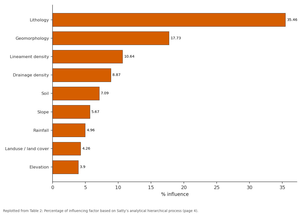
% influence = (Satty Scale/sum)*100: Lithology vs Geomorphology vs Lineament density vs Drainage density vs Soil
Replotted from Table 2 (page 4) of the original paper. Every bar is the paper's own table value.
View source evidence ↗Figures & tables
From the original paper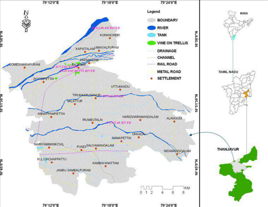 Figure 1
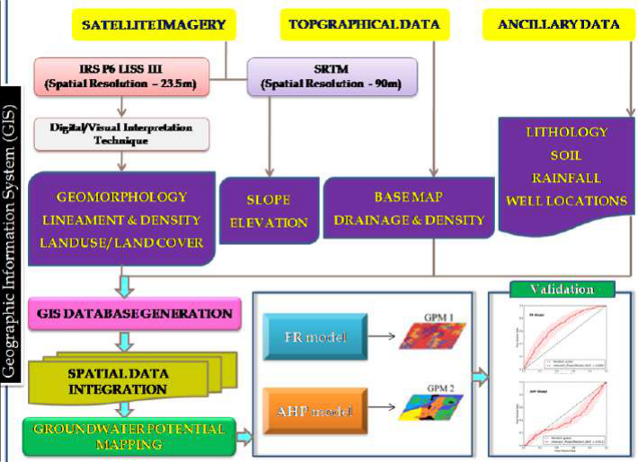 Figure 2
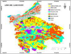 Figure 3
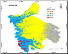 Figure 3
 Table 1
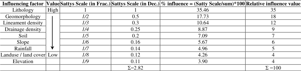 Table 2
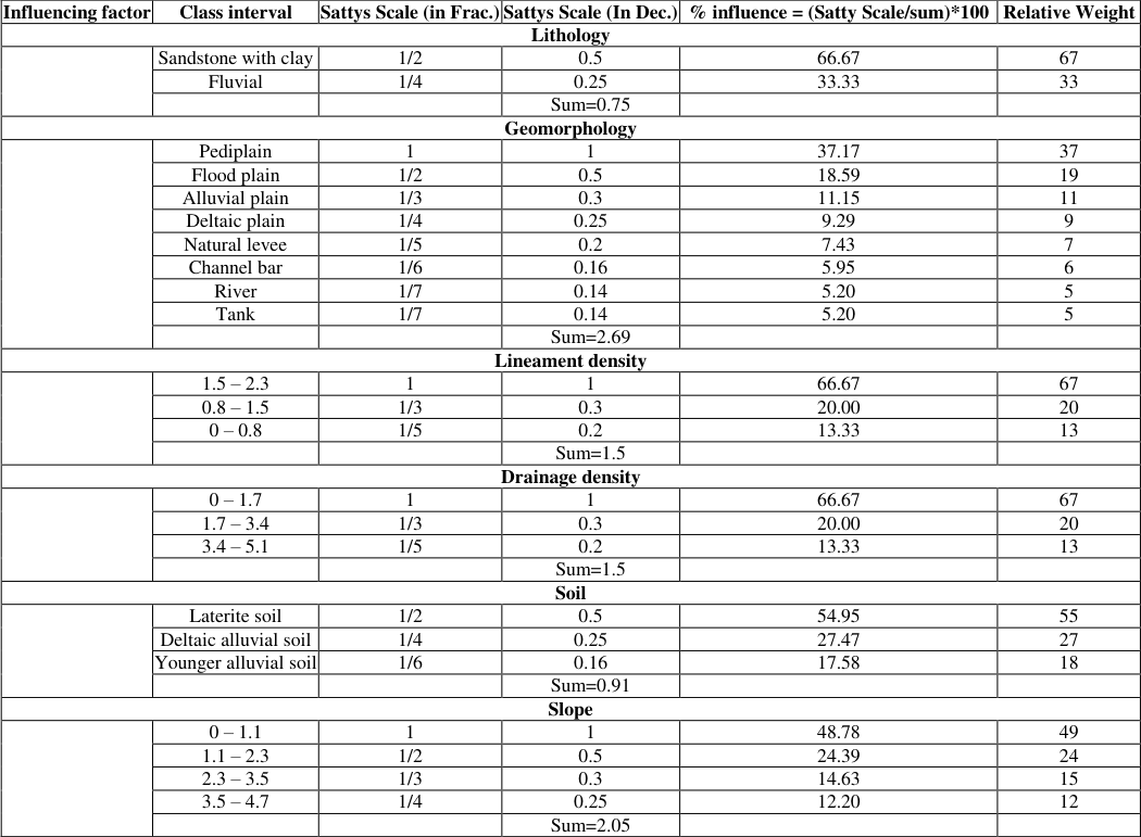 Table 3
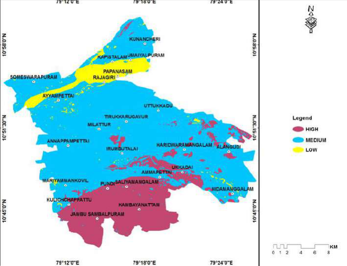 Figure 4
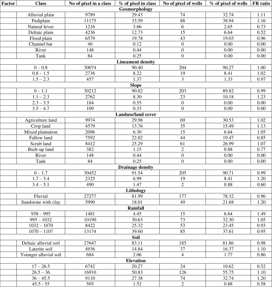 Table 4
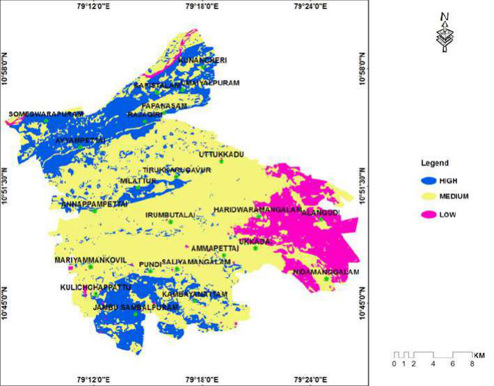 Figure 5
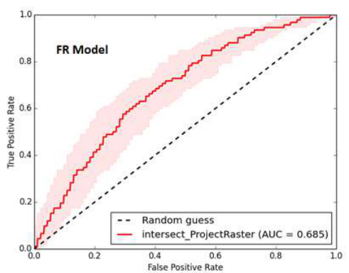 Figure 6
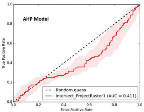 Figure 6
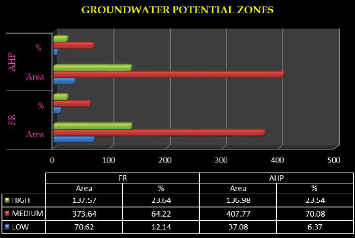 Figure 7
Introduction
Water is an important constituent of all forms of life; groundwater is a most important natural resource of the earth and is required in sufficient quantity and acceptable quality to meet the ever increasing demand for various domestic, agricultural and industrial processing operations. Thus, groundwater is emerging as a formidable poverty reduction tool in developing countries and can be delivered to poor communities far more cheaply, quickly and easily than the conventional canal irrigation water (IWMI, 2001) [14] . The significant contribution made for Green Revolution and also as primary reliable source of irrigation during drought years has further strengthened the people's faith in utilization of groundwater as a dependable source (CGWB, 2013) [9] . Groundwater targeting is a very difficult task due to their typical hydrological properties of unconfined and fractured aquifer conditions (Basavarajappa et al. 2013) [7] . It is possible to identify the groundwater potential zones by observing the terrain features like geological structures, geomorphic units and hydrologic characteristics through both high resolution satellite images and field studies along with GIS (Lokesha et al. 2005; Rokade et al. 2007) [17,25] . In the past, several researchers have used RS and GIS techniques for the delineation of groundwater potential zones with successful results (Saraf and [27,24,19,3,12,8] . The identification of groundwater potential zone using remote sensing and GIS techniques involves interpretation of various thematic maps such as hydro geomorphology, land use / land cover, vegetation, lithology, drainage, subsurface lithology, structure, slope etc. which has been used in inferring the occurrence of ground water (Hung et [13,29,28] . Several studies have been applied using index-based methods for assessing groundwater potential mapping (Prasad et al. 2008; Dar et al. 2011) [23,10] . In some studies, probabilistic models such as frequency ratio (Oh et al., 2011; Naghibi et al., 2016) [20,18] , weight of evidence (Lee et al. 2012; Al-Abadi 2015) [16,2] , logistic regression (Ozdemir 2011; Pourtaghi and Pourghasemi 2014) [21,22] , and analytical hierarchy process (Adiat et al. 2012; Kaliraj et al. 2014) [1,15] have been used for groundwater potential zone mapping. As mentioned above, groundwater studies have become crucial not only for targeting groundwater potential zone, but also for monitoring and conserving this vital resource. The main objective of the present study was to assess and compare the results of groundwater potential zone maps using the analytical hierarchy process and frequency ratio model in the Papanasam Taluk, Thanjavur district.
Study area
The study area is situated in the northern part of Thanjavur district; it is one of the eight taluks. Papanasam taluk is one of the most important agricultural based areas, which is lying in Cauvery river deltaic region. The branch of the Cauvery and Coleroon Rivers are bounded this taluk. It occurs in between Kumbakonam and Thanjavur, Thiruvaiyaru taluk to the eastern and western direction. Papanasam taluk is located at North latitude of 10°70′19″ to 11°00′30″ and East longitude of 79°11′64″ to 79°44′70″ and cover the Survey of India topographic sheet no. 58 N/1, N/2,N/6, N/5, M/8, in 1:50,000 scale and shown in Fig 1 . The talk encompasses eleven blocks and the total areal extent is about 581.83sq.km.
Methodology and data preparation
The methodology adopted for the identification of groundwater potential zone mapping using analytical hierarchy process (AHP) and frequency ratio (FR) model is described in Fig 2 . The data such as remote sensing data, topographical data and existing map from various departments are collected for the successful completion of the study. The basic information about the study area, drainage and density are derived using topographical data 58 M/8, N/1, N/2, N/5, and N6 on 1:50,000 scale. The well location data were collected from the central groundwater board (CGWB) department. Various thematic databases like Lithology, Geomorphology, Lineament density, Drainage density, Soil, Slope, Rainfall, Landuse/Land cover and Elevation were generated to identify groundwater potential zones (Fig. 3). The factors like geomorphology, lineament and density, and landuse and land cover, were interpreted from IRS-LISS III satellite data. The slope and elevation factors were derived in GIS environment using Shuttle Radar Topographic Mission (SRTM) data. The lithology map of the study area was prepared from geological society of India map source. The soil map of the study area was prepared from published maps of soil survey department. The rainfall map of the study area which is prepared from station data (non-spatial). A vector to raster conversion of all the thematic maps with 23.5 x 23.5 m pixel size. The total study area covers 33, 267 pixels, and the total number of well location points is 323 pixels. Among the spring wells, 70% (226 wells) were selected as training data set for GWPZ mapping using FR model and remaining 30% (97 wells) were selected as testing data set for validation of the model. The groundwater potential zones were obtained by overlaying all the thematic maps in terms of frequency ratio and analytical hierarchical process methods using spatial analysis tools in GIS environment. Finally, the different methods of output results of the groundwater potential map are classified into three classes viz. high, medium, and low potential zones.
Analytical Hierarchy Process model
AHP is a widely used multi-criteria decision making MCDM technique in the field of natural resources and environmental management. The analytical hierarchical process was used to determine the weights of the thematic layers (Saaty 1980) [26] . The comparison ratings are in Saaty's 1-9 scale (Saaty 1980) [26] . In order to determine the weight of each thematic layer, the higher the weight, the more important the corresponding criterion. Next, for a fixed criterion, the AHP assigns a score to each option according to the decision maker's pair wise comparisons of the options based on that criterion. The higher the score, the better the performance of the option with respect to the considered criterion. The AHP combines the criteria weights and the option scores, thus determining a global score for each option, and a consequent ranking. The global score for a given option is a weighted sum of the scores it obtained with respect to all the criteria. The table 1 shows the procedure of assigning weightage for each parameter and classes within the parameter based on the importance of it. The value 9 in the table shows higher important while 1/9 shows the least important while 1 shows the equal weight of a parameter or a class. Based on these weightage criteria each parameter in the study has been classified. The weightage of each main parameter has been determined and shown in Table 2, further, the weightage for the subclass of main parameters have been assigned as mention in Table 3. ---------------------------
| Influencing factor | Class interval | Sattys Scale (in Frac.) | Sattys Scale (In Dec.) | % influence = (Satty Scale/sum)*100 | Relative Weight |
|---|---|---|---|---|---|
| Lithology | |||||
| Sandstone with clay | 1/2 | 0.5 | 66.67 | 67 | |
| Fluvial | 1/4 | 0.25 | 33.33 | 33 | |
| Sum=0.75 | |||||
| Geomorphology | |||||
| Pediplain | 1 | 1 | 37.17 | 37 | |
| Flood plain | 1/2 | 0.5 | 18.59 | 19 | |
| Alluvial plain | 1/3 | 0.3 | 11.15 | 11 | |
| Deltaic plain | 1/4 | 0.25 | 9.29 | 9 | |
| Natural levee | 1/5 | 0.2 | 7.43 | 7 | |
| Channel bar | 1/6 | 0.16 | 5.95 | 6 | |
| River | 1/7 | 0.14 | 5.20 | 5 | |
| Tank | 1/7 | 0.14 | 5.20 | 5 | |
| Sum=2.69 | |||||
| Lineament density | |||||
| 1.5 – 2.3 | 1 | 1 | 66.67 | 67 | |
| 0.8 – 1.5 | 1/3 | 0.3 | 20.00 | 20 | |
| 0 – 0.8 | 1/5 | 0.2 | 13.33 | 13 | |
| Sum=1.5 | |||||
| Drainage density | |||||
| 0 – 1.7 | 1 | 1 | 66.67 | 67 | |
| 1.7 – 3.4 | 1/3 | 0.3 | 20.00 | 20 | |
| 3.4 – 5.1 | 1/5 | 0.2 | 13.33 | 13 | |
| Sum=1.5 | |||||
| Soil | |||||
| Laterite soil | 1/2 | 0.5 | 54.95 | 55 | |
| Deltaic alluvial soil | 1/4 | 0.25 | 27.47 | 27 | |
| Younger alluvial soil | 1/6 | 0.16 | 17.58 | 18 | |
| Sum=0.91 | |||||
| Slope | |||||
| 0 – 1.1 | 1 | 1 | 48.78 | 49 | |
| 1.1 – 2.3 | 1/2 | 0.5 | 24.39 | 24 | |
| 2.3 – 3.5 | 1/3 | 0.3 | 14.63 | 15 | |
| 3.5 – 4.7 | 1/4 | 0.25 | 12.20 | 12 | |
| Sum=2.05 |
Table text extracted from the original PDF; superscript letters are shown inline. The original table image is below.
View original table image
| Influencing factor | Value | Sattys Scale (in Frac.) | Sattys Scale (in Dec.) | % influence = (Satty Scale/sum)*100 | Relative influence value |
|---|---|---|---|---|---|
| Lithology | High | 1 | 1 | 35.46 | 35 |
| Geomorphology | 1/2 | 0.5 | 17.73 | 18 | |
| Lineament density | 1/3 | 0.3 | 10.64 | 12 | |
| Drainage density | 1/4 | 0.25 | 8.87 | 9 | |
| Soil | 1/5 | 0.2 | 7.09 | 7 | |
| Slope | 1/6 | 0.16 | 5.67 | 6 | |
| Rainfall | 1/7 | 0.14 | 4.96 | 5 | |
| Landuse / land cover | Low | 1/8 | 0.12 | 4.26 | 4 |
| Elevation | 1/9 | 0.11 | 3.90 | 4 | |
| Σ=2.82 | Σ =100 |
Table text extracted from the original PDF; superscript letters are shown inline. The original table image is below.
View original table image
| 1/9 | 1/7 | — | — | 1/5 | 1/3 | 1 | 3 | 5 | 7 | — | 9 |
|---|---|---|---|---|---|---|---|---|---|---|---|
| Extremely | Very strongly | Strongly | Moderately | Equally | Moderately | Strongly | Very strongly | Extremely | |||
| Less important | ---------------------------- | Equal 1 | -------------------------- | More important |
Table text extracted from the original PDF; superscript letters are shown inline. The original table image is below.
View original table image
More important Source: Satty (1980) [26] Note: 1/8, 1/6, 1/4, 1/2, 2,4,6,8 can also be used if more number of classes exits
Weighted Overlay Analysis
Based on the weightages the Satty's Analytical Hierarchical process the GIS analysis has been carried out, integration of thematic maps for overlay analysis using GIS environment. After integration of all the thematic layer, the GWPI had a minimum value of 151, and a maximum value of 394, with a mean value of 291.32 and a standard deviation of 42.61.
Further, the result of overlay analysis has been classified into three classes as high, medium, and low potential zones and shown in Fig. 4. From the result of classification it has been found that, 136.98 km 2 areas are having high, 407.77 km 2 area is having medium, and 37.08 km 2 having low for groundwater potential zones.
Frequency Ratio model
Frequency ratio (FR) model as bivariate statistical technique can be utilized as a simple tools for geospatial valuation and computation of the probabilistic association between dependent variable and independent variables. The method has been used for groundwater spring potential mapping by Ozdemir (2011) [21] . The spatial relationships between groundwater well locations and each factor contributing groundwater occurrence. For groundwater potential analysis, the calculated and extracted factors were converted to a 23.5 x 23.5 m 2 grid using ArcGIS software. In the study area, the total number of pixels was 33,267, and the number of well location pixels was 323. Among the spring wells, 70% (226 wells) were selected as training data set for GWPZ mapping using FR model and remaining 30% (97 wells) were selected as testing data set for validation of model on the basis of random dividing method (Lee et al. 2012) [16] . The correlation of coefficients was calculated from the analysis of the relationship between the well location and the relevant factors. The rating of each factor's type or range was assigned from the relationship between distribution of groundwater well location and each groundwater conditioning factor's. To compute the frequency value in each class of the groundwater-related factors can be expressed based on the equation.
FR (1)
Where, FR is the frequency ratio of the class of factor, W is a number of pixels of well locations for each class of thematic maps; TW is a number of total pixels of well in the study area. CP is a number of pixels in each thematic class and TP is a total number of pixels in the study area. The calculated values have given in Table-4. In the FR model, the FR value of each class in a thematic layer was considered as the weight of that particular class in thematic parameters to determine groundwater potentiality. The accuracy of the FR model was validated using R-index method.
Data Integration
The calculated frequency ratio values were added to the attribute table of each thematic layer. These thematic layers were converted into a raster layer based on the frequency ratio field values. All the raster themes were integrated in the GIS environment by using raster calculator options in spatial analyst tool. The data integration has done to calculate the groundwater potential index by using the following equation. GWPIFR = ∑ (GEOMFR + LDFR + SLFR + Lu_LcFR + DDFR + LIFR + RFFR + SOFR +ELFR)
(2) Where, GWPIFR = Groundwater Potential Index using frequency ratio method. GEOMFR = freqency ratio of geomorphology; LDFR = frequency ratio of lineament density; SLFR = frequency ratio of slope; Lu_LcFR = frequency ratio of landuse/land cover; DDFR = frequency ratio of drainage density; LIFR = freqency ratio of lithology; RFFR = frequency ratio of rainfall; SOFR = freqency ratio of soil; ELFR = frequency ratio of elevation. After integration of all the raster layer, the GWPI had a minimum value of 6.24, and a maximum value of 11.12, with a mean value of 9.0 and a standard deviation of 0.73. The range of minimum and maximum values were equally divided into three categories and classified as high, medium, and low potential classes and the groundwater potential zone map generated based on the frequency ratio model and shown in Fig 5 . Based on the frequency ratio of the groundwater potential classes, 23.64% of the area fall in high, 64.22% of the area comes under the medium, and 12.14% of the area comes in low potential categories. [11,21,4,5] . In this study, the output map for groundwater potential were validated through the receiver operating characteristic (ROC) analysis by comparing the 97 (30%) existing well locations for validation purposes. The ROC curve of the groundwater potential zone maps obtained by the AHP and FR models and shown in Fig. 6. These curves indicate that the FR model (AUC=68.5%) performs better than AHP model (AUC=41.1%) model. Therefore, it can be seen that the FR and AHP models applied in this study showed reasonably good accuracy in spatial predicting of groundwater potential.
Summary and Conclusion
Generally various methods have been applied for regional groundwater potential assessment globally. In this study, analytical hierarchy process and frequency ratio models were applied by considering nine thematic layers such as lithology, geomorphology, lineament density, drainage density, soil, slope, rainfall, land use/land cover and elevation in order to identify groundwater potential zones. AHP multi-criterion analysis and FR models were used to evaluate the weight and rating values for thematic layers and their sub-classes respectively. All the thematic layers to be integrated and analyzed in the GIS environment. Subsequently, the groundwater potential index were calculated and reclassified in to high, medium and low groundwater potential zones. The result of FR model revealed that, around 462.39 km 2 (79.47%) area is high, 118.65 km 2 (20.39%) area is medium and 0.79 km 2 (0.14%) area is low potential zones. From the AHP model, mapping of groundwater potential zone shows that 136.98 km2 (23.54%) of the study areas are high and 407.77 km2 (70.08%) are medium and 37.08 km2 (6.37%) of the area remote chance of potential zones and shown in Fig. 7. The model's outcomes acquired in this research were validated with the distribution of existing validation purposes of groundwater wells locations using ROC curve method. The validation of the results showed that the FR model (AUC=68.5%) performs better than AHP (AUC=41.1%) models. The higher value of the AUC indicates the highly successful nature of the techniques used in this study. Hence, the outcomes attained from the present study indicated that the FR and AHP model can offer an influential tool for delineation of the groundwater resource. The results of groundwater potential maps can be useful for planners and engineers in water resource management and land use planning of the study area.
Figures and tables from the paper
| Factor | Class | No of pixel in a class | % of pixel in class | No of pixel of wells | % of pixel of wells | FR ratio |
|---|---|---|---|---|---|---|
| Geomorphology | ||||||
| Alluvial plain | 9789 | 29.43 | 74 | 32.74 | 1.11 | |
| Pediplain | 11175 | 33.59 | 88 | 38.94 | 1.16 | |
| Natural levee | 1216 | 3.66 | 6 | 2.65 | 0.73 | |
| Deltaic plain | 4236 | 12.73 | 15 | 6.64 | 0.52 | |
| Flood plain | 6579 | 19.78 | 43 | 19.03 | 0.96 | |
| Channel bar | 40 | 0.12 | 0 | 0.00 | 0.00 | |
| River | 148 | 0.44 | 0 | 0.00 | 0.00 | |
| Tank | 84 | 0.25 | 0 | 0.00 | 0.00 | |
| Lineament density | ||||||
| 0 – 0.8 | 30074 | 90.40 | 204 | 90.27 | 1.00 | |
| 0.8 – 1.5 | 2736 | 8.22 | 19 | 8.41 | 1.02 | |
| 1.5 – 2.3 | 457 | 1.37 | 3 | 1.33 | 0.97 | |
| Slope | ||||||
| 0 – 1.1 | 30212 | 90.82 | 203 | 89.82 | 0.99 | |
| 1.1 – 2.3 | 2762 | 8.30 | 23 | 10.18 | 1.23 | |
| 2.3 – 3.5 | 184 | 0.55 | 0 | 0.00 | 0.00 | |
| 3.5 – 4.7 | 109 | 0.33 | 0 | 0.00 | 0.00 | |
| Landuse/land cover | ||||||
| Agriculture land | 9974 | 29.98 | 69 | 30.53 | 1.02 | |
| Crop land | 4579 | 13.76 | 35 | 15.49 | 1.13 | |
| Mixed plantation | 2096 | 6.30 | 15 | 6.64 | 1.05 | |
| Fallow land | 7592 | 22.82 | 44 | 19.47 | 0.85 | |
| Scrub land | 8412 | 25.29 | 61 | 26.99 | 1.07 | |
| Built-up land | 382 | 1.15 | 2 | 0.88 | 0.77 | |
| River | 148 | 0.44 | 0 | 0.00 | 0.00 | |
| Tank | 84 | 0.25 | 0 | 0.00 | 0.00 | |
| Drainage density | ||||||
| 0 – 1.7 | 30452 | 91.54 | 205 | 90.71 | 0.99 | |
| 1.7 – 3.4 | 2325 | 6.99 | 19 | 8.41 | 1.20 | |
| 3.4 – 5.1 | 490 | 1.47 | 2 | 0.88 | 0.60 | |
| Lithology | ||||||
| Fluvial | 27277 | 81.99 | 177 | 78.32 | 0.96 | |
| Sandstone with clay | 5990 | 18.01 | 49 | 21.68 | 1.20 | |
| Rainfall | ||||||
| 958 – 995 | 1481 | 4.45 | 15 | 6.64 | 1.49 | |
| 995 – 1032 | 10190 | 30.63 | 73 | 32.30 | 1.05 | |
| 1032 – 1070 | 8422 | 25.32 | 53 | 23.45 | 0.93 | |
| 1070 – 1107 | 13174 | 39.60 | 85 | 37.61 | 0.95 | |
| Soil | ||||||
| Deltaic alluvial soil | 27647 | 83.11 | 185 | 81.86 | 0.98 | |
| Laterite soil | 4936 | 14.84 | 37 | 16.37 | 1.10 | |
| Younger alluvial soil | 684 | 2.06 | 4 | 1.77 | 0.86 | |
| Elevation | ||||||
| 17 – 26.5 | 6742 | 20.27 | 24 | 10.62 | 0.52 | |
| 26.5 – 36 | 16910 | 50.83 | 126 | 55.75 | 1.10 | |
| 36 – 45.5 | 9110 | 27.38 | 74 | 32.74 | 1.20 | |
| 45.5 - 55 | 505 | 1.52 | 2 | 0.88 | 0.58 |
Table text extracted from the original PDF; superscript letters are shown inline. The original table image is below.
View original table image
References
29 in the original paper- Adiat KAN, Nawawi MNM, Abdullah K. Assessing the accuracy of GIS-based elementary multi criteria decision analysis as a spatial prediction tool-A case of predicting potential zones of sustainable groundwater resources. Journal of Hydrology 2012;440:75-89.
- Al-Abadi AM. Groundwater potential mapping at north eastern Wasit and Missan governorates, Iraq using a data-driven weights of evidence technique in framework of GIS. Environmental Earth Sciences 2015;74:1109-1124.
- Anbazhagan S, Jothibasu A. Geo informatics in groundwater potential mapping and sustainable development: a case study from southern India. Hydrological Sciences Journal 2016;61(6):1109-1123.
- Andualem TG, Demeke GG. Groundwater potential assessment using GIS and remote sensing: A case study of Guna tana landscape, upper blue Nile Basin, Ethiopia. Journal of hydrology: Regional studies 2019;24:100610.
- Arfan Arshad, Zhijie Zhang, Wanchang Zhang, Adil Dilawar. Mapping favourable groundwater potential recharge zones using a GIS-based analytical hierarchical process and probability frequency ratio model: A case study from an agro-urban region of Pakistan. Geoscience Frontiers 2020;11:1805-1819.
- Baeza C, Corominas J. Assessment of shallow landslide susceptibility by means of multivariate statistical techniques. Earth Surface Processes and Landforms 2001;26:1251-1263.
- Basavarajappa HT, Dinakar S, Satish MV, Nagesh D, Balasubramanian A, Manjunatha MC. Delineation of Groundwater Potential Zones in Hard Rock Terrain of Kollegal Shear Zone (KSZ), South India, using Remote Sensing and GIS. International Journal of Earth Sciences and Engineering 2013;6(5):1185-1194.
- Biswajit Das, Subodh Chandra Pal. Assessment of groundwater recharge and its potential zone identification in groundwater-stressed Goghat-I block of Hugli District, West Bengal, India. Environment, Development and Sustainability 2019;22:5905-5923.
- CGWB. Master Plan for Artificial Recharge to Groundwater in India. Ministry of Water Resources, Govt. of India 2013.
- Dar IA, Sankar K, Dar MA. Deciphering groundwater potential zones in hard rock terrain using geospatial technology. Environmental Monitoring and Assessment 2011;173(1-4):597-610.
- Das S. Comparison among influencing factor, frequency ratio, and analytical hierarchy process techniques for groundwater potential zonation in Vaitarna basin, Maharashtra, India. Groundwater for Sustainable Development 2019;8:617-629.
- Hema C, Nair Padmalal D, Ammini Joseph Vinod PG. Delineation of Groundwater Potential Zones in River Basins Using Geospatial Tools-an Example from Southern Western Ghats, Kerala, India. Journal of Geovisualization and Spatial Analysis 2017;1(5):1-2.
- Hung LQ, Dinh NQ, Batelaan O, Tam VT, Lagrou D. Remote sensing and GIS-based analysis of cave development in the Suoimuoi Catchment (Son La-NW Vietnam). Journal of Cave and Karst Studies 2002;64 (1):23-33.
- IWMI. The Strategic Plan for IWMI 2000-2005 (Colombo, Sri Lanka: International Water Management Institute) 2001.
- Kaliraj S, Chandrasekar N, Magesh NS. Identification of potential groundwater recharge zones in Vaigai upper basin, Tamil Nadu, using GIS-based analytical hierarchical process (AHP) technique. Arabian Journal of Geosciences 2014;7:1385-1401.
- Lee S, Song KY, Kim Y, Park I. Regional groundwater productivity potential mapping using a geographic information system (GIS) based artificial neural network model. Hydrogeology Journal 2012;20(8):1511-1527.
- Lokesha N, Gopalakrishna GS, Honne Gowda H, Gupta AK. Delineation of groundwater potential zones in a hard rock terrain of Mysore district, Kamatak using IRS data and GIS techniques. Journal of the Indian society of Remote Sensing 2005;33(3):405-412.
- Naghibi SA, Pourghasemi HR, Dixon B. Groundwater spring potential using boosted regression tree, classification and regression tree, and random forest machine learning models in Iran. Environmental Monitoring and Assessment 2016;188:44.
- Neelakantan R, Yuvaraj S. Evaluation of groundwater using geospatial data -a case study from Salem taluk, Tamil nadu, India. International Journal of Remote Sensing & Geoscience 2012;1(2):7-12.
- Oh HJ, Kim YS, Choi JK, Park E, Lee S. GIS mapping of regional probabilistic groundwater potential in the area of Pohang City, Korea. Journal of Hydrology 2011;399:158-172.
- Ozdemir, Adnan. GIS-based groundwater spring potential mapping in the Sultan Mountains (Konya, Turkey) using frequency ratio, weights of evidence and logistic regression methods and their comparison. Journal of Hydrology 2011;411:290-308.
- Pourtaghi ZS, Pourghasemi HR. GIS-based groundwater spring potential assessment and mapping in the Birjand Township, southern Khorasan Province Iran. Hydrogeology 2014;22:643-662.
- Prasad RK, Mondal NC, Banerjee P, Nandakumar MV, Singh VS. Deciphering potential groundwater zone in hard rock through the application of GIS. Environmental Geology 2008;55:467-475.
- Rai B, Tiwar A, Dubey VS. Identification of groundwater prospective zones by using remote sensing and geoelectrical methods in Jharia and Raniganj coalfields, Dhanbad district, Jharkhand state. Journal of Earth System Sciences 2005;114(5):515-522.
- Rokade VM, Kundal P, Joshi AK. Groundwater potential modeling through remote sensing and GIS: a case study from Rajura Taluka, Chand rapur district, Maharashtra. Journal of the Geological Society of India 2007;69:943-948.
- Saaty TL. The analytic Hierarchy Process: planning, priority setting, resource allocation. McGraw-Hill, New York 1980, 287.
- Saraf AK, Choudhury PR. Integrated remote sensing and GIS for groundwater exploration and identification of artificial recharge sites. International Journal of Remote Sensing 1998;19:1825-1841.
- Shaban A, Khawlie M, Abdallah C. Use of remote sensing and GIS to determine recharge potential zones: the case of Occidental Lebanon. Hydrogeology Journal 2006;14(4):433-443.
- Xiuwan C. Using remote sensing and GIS to analyse land cover change and its impacts on regional sustainable development. International Journal of Remote Sensing 2002;23(1):107-124.
Cited by 8
From OpenAlex, OpenCitations and reference lists read by Scinovex
- Integrated GIS-based approach for groundwater potential mapping in arid regions: A case study of Kenadsa-Bechar using AHP and frequency ratio methods ↗
Abdeldjalil Belkendil, Mohammed Habi, Manel Yakhlefoune, Sarra Ameri, Abderrahmane Mekkaoui, Aqil Tariq et al. · Groundwater for Sustainable Development · 2025
Groundwater potential studies are vital for sustainable water resource management in arid regions facing severe water scarcity such as the Kenadsa-Bechar area in northwestern Bechar province, Algeria. This study integrates the Analytical Hierarchy Process (AHP) and Frequency Ratio FR methods integrated with Geographic Information Systems (GIS) to map groundwater potential zones (GWPZ) and support agricultural resilience in a region with…
❝ 17PDF - Determination of the levels of heavy metals and physicochemical properties of borehole water within selected mining sites in Ebonyi state, Nigeria ↗
David Okechukwu Okeke, Jonathan C. Ifemeje, Victor Chukwuemeka Eze · International Journal of Chemical and Biological Sciences · 2021
The level of heavy metals (Pb, Cd, As, Cr, Ni, Co, Zn) and physicochemical parameters in borehole water sources within selected mining sites in Ebonyi State, Nigeria were determined using FS240AA Atomic Absorption Spectrophotometer (AAS) according to the method of American Public Health Association (APHA). Water samples were collected from Enyigba mining site, Ikwo mining site, Ameri Amekamining site, Izza
- Challenges for groundwater-irrigated agriculture and management opportunities in Punjab province of Pakistan
Ghulam Zakir-Hassan, Faiz Raza Hassan, JF Punthakey, Ghulam Shabir · International Journal of Agriculture and Nutrition · 2022
Pakistan has one of the world’s largest contiguous irrigation canal networks which was initiated by the British during the early nineteenth century, and its continuous expansion significantly altered the hydrological balance of the Indus River Basin (IRB) in Pakistan. During the pre-irrigation era, the water table in the IRB was very deep which rose up with the introduction of canal network. Seepage from the earthen canals caused the dual menace of waterlogging and salinity and different Salinity Control and Reclamation Projects (SCARPs) were implemented. With the growing food and fiber requir
- Potential natural obstacles to groundwater engineering ↗
N.H. Farhat, Walid Sleiman · Journal of Civil Engineering and Applications · 2023
Countries have constantly experienced problems with water resources: much, little, polluted, variable. Over generations, humankind has tried to manage these water resources problems by intervening in its natural courses through redistribution, storage, and regulation. Management and exploitation resulted in systematic knowledge of the behavior of surface and underground water. The center of importance subsequently shifted to groundwater at the beginning
- Groundwater potential and recharge zones mapping using remote sensing and GIS for Kadegaon Taluka, Maharashtra, India ↗
Digvijay S Shinde, DB Desai, JS Lambe, Abhijit M Zende · International Journal of Civil Engineering and Architecture Engineering · 2022
Year by year the water is becoming the scare source all over the world. Water resources available on earth are in the two forms namely surface water and ground water. According to the study of scientist the total volume of the ground water is very less as compared to the total water available in the globe. There are many areas
- Problems and prospects of water resources in Karnataka
Aditya V Machnoor, DS Gurjar · International Journal of Agriculture and Food Science · 2023
India's annual precipitation is thought to be around 4000 billion cubic metres (bcm) and its potential water supply is 1869 bcm. The overall utilisable water resource potential is 1137 bcm, made up of 690 bcm of surface water and 447 bcm of groundwater due to topographical and other limitations. In India, the yearly water availability per person was around 1544 cubic metres in 2011, but has since decreased owing to population growth. A country is deemed to be under water stress if its per capita annual renewable water supply falls below 1700 m3, according to the widely used Falkenmark Index (J
- Evaluation of water resources: A case study of Rohtak district, Haryana ↗
Jyoti Devi, Sandeep Kumar, Sunil Kumar · International Journal of Communication and Information Technology · 2023
Water is one of the most important natural resources for life. Because of the rapid increase in population, urbanization, and industrialization, the demand for water to meet various needs is constantly increasing. Water that is present below the Earth's surface and fills any gaps in the soil or geologic strata is known as groundwater. It is additionally known as subsurface
- Impact of solid waste dumping yard on ground water
R. Das, Arvind K Dwivedi · International Journal of Biology Sciences · 2023
Municipal and industrial trash is frequently disposed of in solid waste dumps or landfills. However, these dump sites have a substantial impact on the quality and availability of groundwater, which is essential for supporting ecosystems and providing for human requirements in terms of water. In this article, the effect of solid waste disposal yards on groundwater is examined, along with any possible repercussions. Leachate, a fluid that introduces contaminants into the groundwater, can occur as a result of poor trash compaction, inadequate liners or barriers, or incorrect management of dumping