
Research article · 2020 · Full text
International Journal of Statistics and Applied MathematicsThe logistic-Rayleigh distribution with properties and applications
Volume 5(6) · Pages 12–19 · DOI: 10.22271/maths.2020.v5.i6a.603 ↗
Research areasStatistical Distribution Estimation and ApplicationsInsurance, Mortality, Demography, Risk Management
Abstract
Author-writtenIn this article, we have presented a two-parameter univariate continuous distribution called Logistic-Rayleigh distribution. We have discussed some mathematical and statistical properties of the distribution, such as the cumulative distribution function, probability density function and hazard rate function, survival function, quantile function, the skewness, and kurtosis measures. The model parameters of the proposed distribution are estimated using three well-known estimation methods, namely maximum likelihood estimation (MLE), least-square estimation (LSE), and Cramer-Von-Mises estimation (CVME) methods. The goodness of fit of the purposed distribution is also evaluated by fitting it in comparison with some other existing distributions using a real data set.
Summary
Source-checkedPlain-language reading of the full paper, prepared with AI and checked against the text. Each point links to the authors' own words.
Why it matters
- Researchers often generalize standard probability distributions because existing models may not provide an optimal fit for survival data. View evidence ↗
- A survival model capable of representing multiple failure rate shapes (increasing, decreasing, bathtub, and inverted bathtub) is highly useful for fitting diverse lifetime data sets. View evidence ↗
- The logistic distribution is useful for analyzing extreme events because its tails are wider than those of a normal distribution. View evidence ↗
The question
- The study aims to create a more flexible distribution for lifetime data by adding a single parameter to the Rayleigh distribution. View evidence ↗
What they did
- The authors developed the Logistic-Rayleigh (L-R) distribution following the approach established by Lan and Leemis (2008). View evidence ↗
- The model parameters were estimated using three methods: maximum likelihood estimation (MLE), least-square estimation (LSE), and Cramer-Von-Mises estimation (CVME). View evidence ↗
- The proposed distribution was tested using a real dataset consisting of failure times for 59 conductors from an accelerated life test. View evidence ↗
What they found
- The L-R distribution was found to be flexible and characterized by an inverted bathtub-shaped hazard function. View evidence ↗
- The authors concluded that maximum likelihood estimation (MLE) provided better parameter estimates than LSE and CVME. View evidence ↗
- The L-R distribution demonstrated a better fit than competing models, as evidenced by minimum test statistic values and higher p-values. View evidence ↗
- The L-R model outperformed the Gompertz (GZ) model across all information criteria, with a lower AIC (226.4098 vs 238.3480) and lower BIC (230.5649 vs 242.5031). View evidence ↗
What it means
- The authors suggest that the L-R distribution can serve as a viable alternative for applications in applied statistics, probability theory, and survival analysis. View evidence ↗
Visual summary
3 visualsIllustrations explain the paper; charts are replotted from the paper's own table values.
Conceptual Construction of L-R Distribution
AI-generated conceptual illustration (Abstract mathematical probability density curves). It explains the idea and does not show study data.
View source evidence ↗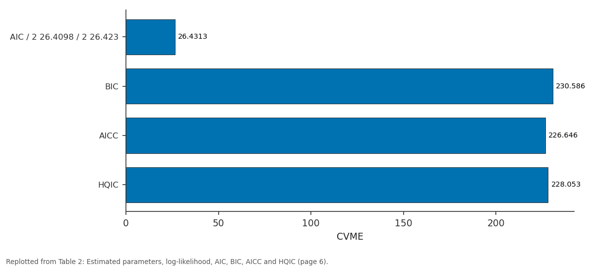
CVME: AIC / 2 26.4098 / 2... vs BIC vs AICC vs HQIC
Replotted from Table 2 (page 6) of the original paper. Every bar is the paper's own table value.
View source evidence ↗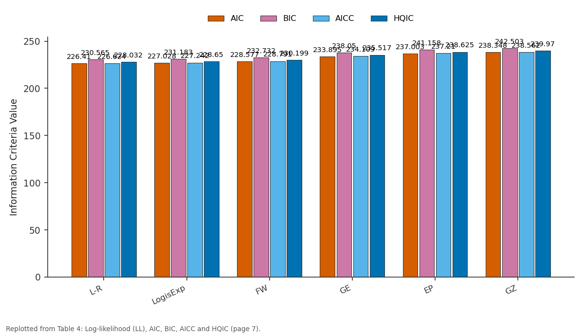
AIC and BIC and more: L-R vs LogisExp vs FW vs GE vs EP
Replotted from Table 4 (page 7) of the original paper. Every bar is the paper's own table value.
View source evidence ↗Figures & tables
From the original paper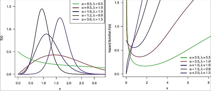 Figure 1
 Table 1
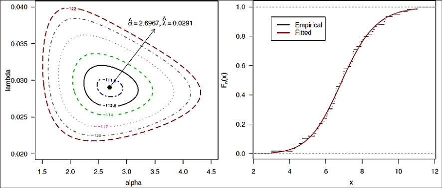 Figure 2
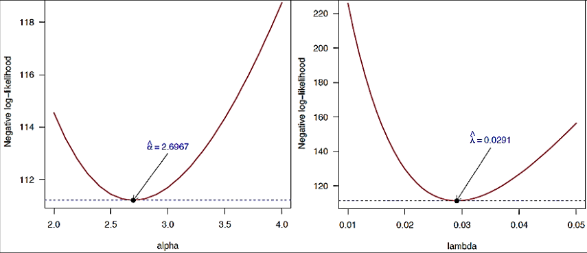 Figure 3
 Table 2
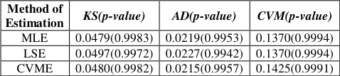 Table 3
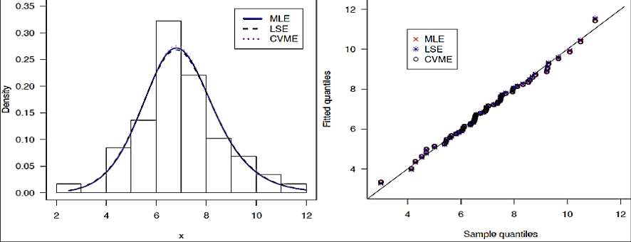 Figure 4
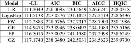 Table 4
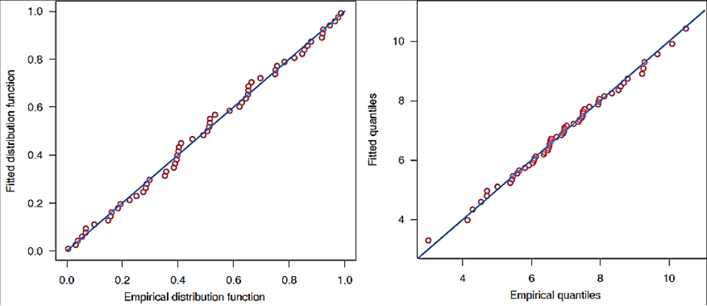 Figure 5
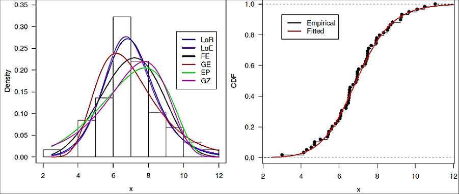 Figure 6
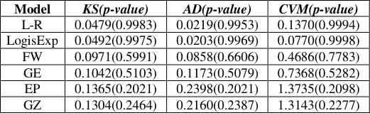 Table 5
Introduction
In most of the literature of probability distributions and applied statistics, it is observed that the study of reliability and survival analysis in various fields of applied statistics and life sciences, the probability distributions are often used. In modelling survival data, existing models do not always reveal a better fit. Hence most of the researchers are interested in generalizing standard distributions and investigating their flexibility and applicability. Usually, these new compounded models produce an improved fit as compared to usual classical survival models. They are obtained by bringing one or more additional shape parameter(s) to the parent distribution. The exponential distribution plays a vital role in analyses of life testing data in statistics and probability theory. It is the probability distribution of the time between events in a Poisson point process, i.e., a process in which events occur independently and continuously at a constant average rate. It is a specific case of the gamma distribution. It is the continuous analogue of the geometric distribution, and it has the key property of being memory less. In addition to being used for the analysis of Poisson point processes, it is found in various other contexts. A compounded survival model that includes different shapes like increasing, decreasing, bathtub-shaped, and inverted Bathtub-Shaped failure rate in a single model would be constructive in survival analysis. Such a model would provide considerable flexibility and goodness of fit for fitting a broad variety of lifetime data sets. Such a survival model might also be taken to determine the distribution class from which the data is selected by constructing a confidence interval over its parameters. The proposed distribution introduced here satisfies these criteria. The Rayleigh was obtained from the amplitude of sound resulting from many important sources by (Rayleigh, 1880) [18] . It is a continuous probability distribution with a wide range of applications such as in reliability analysis, life testing experiments, clinical studies and applied statistics. This distribution is a particular case of the two-parameter Weibull distribution with the shape parameter equal to 2. Important features, including its origin, can be found in the work of (Siddiqui, 1962) [19] , as well as Howlader and Hossian (1995). A non-negative random variable X follows the Rayleigh distribution with scale parameter θ if its probability density function (PDF) is given by [5] , Bivariate generalized Rayleigh distribution by (Abdel-Hady, 2013) [1] , Transmuted Rayleigh distribution by (Merovci, 2013) [12] , generalized Weibull-Rayleigh distribution by (Yahaya & Alaku, 2018) [23] , New Lindley-Rayleigh distribution by (Joshi & Kumar, 2020) [7] , Weibull-Rayleigh distribution by (Merovci & Elbatal, 2015) [11] , transmuted Weibull-Rayleigh distribution by (Yahaya & Ieren, 2017) [24] as well as the Transmuted Inverse Rayleigh distribution studied by (Ahmad et al., 2015) [2] . The logistic distribution is a univariate continuous distribution, and both its PDF and CDF functions have been used in many different areas such as logistic regression, logit models and neural networks. It has been used in the physical sciences, demography, sports modelling, and recently in finance as well as insurance. The logistic distribution has wider tails than a normal distribution, so it is more consistent with the underlying data and provides better insight into the likelihood of extreme events. Let X be a non-negative random variable which follows the logistic distribution with shape parameter θ > 0, and then its cumulative distribution function is given by
and its corresponding PDF is
Tahir et al. (2016) [22] has defined the logistic-X family as a new generating family of continuous distributions produced from a logistic random variable whose density function can be defined as being right-skewed, left-skewed, symmetrical and reversed-J shaped, and can have decreasing, increasing, bathtub and upside-down bathtub hazard rates shaped. Lan and Leemis (2008) [10] have presented an approach to define the logistic compounded model and introduced the logisticexponential survival distribution. This has several useful probabilistic properties for lifetime modelling. Unlike most distributions in the bathtub and upside-down bathtub classes, the logistic-exponential distribution exhibit closed-form density, hazard, cumulative hazard, and survival functions. The survival function of logistic-exponential distribution is
Using the same approach used by (Lan & Leemis, 2008) [10] we have defined the new distribution called Logistic-Rayleigh (L-R) distribution. The main objective of this article is to introduce a more flexible distribution by inserting just one extra parameter to the Rayleigh distribution to attain a better fit for the lifetime data sets. We have discussed some distributional properties and their applicability. The different sections of the proposed study are arranged as follows. In Section 2, we present the Logistic-Rayleigh (L-R) distribution and its various mathematical and statistical properties. We have made use of three well-known estimation methods to estimate the model parameters, namely the maximum likelihood estimation (MLE), least-square estimation (LSE) and Cramer-Von-Mises estimation (CVME) methods. For the maximum likelihood (ML) estimate, we have constructed the asymptotic confidence intervals using the observed information matrix are presented in Section 3. In Section 4, a real data set has been analyzed to explore the applications and capability of the proposed distribution. In this section, we present the estimated value of the parameters and log-likelihood, AIC, BIC and AICC criterion for ML, LSE, and CVME also the goodness of fit of the proposed distribution is also evaluated by fitting it in comparison with some other existing distributions using a real data set. Finally, in Section 5, some concluding remarks are presented.
The logistic-rayleigh (l-r) distribution
Using the same approach used by (Lan & Leemis, 2008) [10] we have defined the new distribution called Logistic-Rayleigh (L-R) distribution. Let X be a non-negative random variable with a positive shape parameter α and a positive scale parameter λ then CDF of logistic-Rayleigh distribution can be defined as
The density of logistic-Rayleigh (LR) distribution with shape parameter α and scale parameter λ is
This CDF function be similar to the log-logistic CDF function with the second term of the denominator being changed in its base to a Rayleigh function; hence we named it Logistic-Rayleigh distribution.
A. Reliability function
The reliability function of Logistic-Rayleigh distribution is
B. Hazard function
The failure rate function of L-R distribution can be defined as,
In Figure 1, we have displayed the plots of the PDF and hazard rate function of L-R distribution for different values of α and λ.
C. Quantile function
Quantile function of Logistic -Rayleigh distribution can be expressed as
D. Median
The median of Logistic-Rayleigh distribution can be expressed as
Here we notice that the median depends upon scale parameter λ only.
E. Skewness and Kurtosis
The measures Skewness and Kurtosis based on quantiles are, Bowley's coefficient of skewness is
And coefficient of kurtosis based on octiles which were defined by (Moors, 1988) [14] is
Methods of estimation
In this section, the parameters of the proposed distribution are estimated by applying some well-known estimation methods which are as follows
Maximum Likelihood Estimation Method
For the estimation of the parameter, the maximum likelihood method is the most commonly used method (Casella & Berger, 1990). Let, 12 , ,..., ; , ,..., , ,..., / ( / )
Differentiating (3.1.1) with respect to α and λ we get,
is the Fisher's information matrix. Using the Newton-Raphson algorithm to maximize the likelihood creates the observed information matrix, and hence the variance-covariance matrix is obtained as,
Hence from the asymptotic normality of MLEs, approximate 100(1-α) % confidence intervals for α and λ can be constructed as, z is the upper percentile of standard normal variate.
Method of Least-Square Estimation (LSE)
Swain et al. (1988) [21] proposed the weighted least square estimators and ordinary least square estimators to estimate the parameters of Beta distributions. Here we have applied the same procedure for the L-R distribution. The least-square estimators of the unknown parameters α and λ of L-R distribution can be obtained by minimizing
with respect to unknown parameters α and λ. Consider ( ) i GX denotes the distribution function of the ordered random variables
is a random sample of size n from a distribution function G(.). The least-square estimators of α and λ say ˆ and respectively, can be obtained by minimizing
with respect to α and λ. Differentiating (3.2.2) with respect to α and λ we get,
Similarly, the weighted least square estimators can be obtained by minimizing
with respect to α and λ. The weights wi are
Hence, the weighted least square estimators of α and λ respectively can be obtained by minimizing,
Method of Cramer-Von-Mises estimation (CVME)
The CVME estimators of α and λ are obtained by minimizing the function
simultaneously we will get the CVM estimators.
Illustration with a real dataset
The data presented below are from an accelerated life test of 59 conductors used by (Nelson & Doganaksoy, 1995) [16] . The failures can occur in microcircuits because of the movement of atoms in the conductors in the circuit; this is referred to as electro-migration. The failure times are in hours, and there are no censored observations. 2, Kumar & Ligges (2011) [8] . The MLEs are calculated directly by using optim() function in R software (R Core Team, 2020) [17] and (Ming, 2019) [13] by maximizing the likelihood function (3.1.1). We have obtained = 2.6967 and = 0.0291 and the corresponding Log-Likelihood value is -111.2045. In Table 1, we have demonstrated the MLE's with their standard errors (SE) and 95% confidence interval for α and λ. We have displayed the graph of the profile log-likelihood function of α and λ in Figure 3 and observed that the MLEs are unique. By using MLE, LSE and CVME methods we estimate the parameter of L-R distribution.
| Parameter | MLE | SE | 95% ACI |
|---|---|---|---|
| alpha | 2.6967 | 0.2983 | (2.1121, 3.2814) |
| lambda | 0.0291 | 0.0018 | (0.0257, 0.0324) |
Table text extracted from the original PDF; superscript letters are shown inline. The original table image is below.
View original table image
For the goodness of fit purpose, we useAkaike information criterion (AIC), Bayesian information criterion (BIC), Corrected Akaike Information Criterion (AICC) and Hannan-Quinn information criterion (HQIC), negative log-likelihood (-LL), a statistic to select the best model among selected models. The expressions to calculate AIC, BIC, AICC and HQIC are listed below:
where the number of parameters is denoted by k and n denotes sample size in the model under consideration. Further, in order to evaluate the fits of the LHC distribution with some selected distributions, we have taken the Kolmogorov-Simnorov (KS), the Anderson-Darling (W) and the Cramer-Von Mises (A 2 ) statistic. These statistics are widely used to compare non-nested models and to illustrate how closely a specific CDF fits the empirical distribution of a given data set. These statistics are calculated as
the xi's being the ordered observations. In Table 2 we have displayed the estimated value of the parameters of Logistic inverse exponential distribution using MLE, LSE and CVME method and their corresponding negative log-likelihood, AIC, BIC, AICC and HQIC information criteria. In order to illustrate the goodness of fit of the Lindley inverse exponential distribution, we have taken some well-known distribution for comparison purpose which are listed blew,
| Method of Estimation | ˆ | ˆ | -LL | AIC | BIC | AICC | HQIC |
|---|---|---|---|---|---|---|---|
| ML | 2.6967 | 0.0291 | 111.2049 | 2 26.4098 | 230.5649 | 226.6241 | 228.0318 |
| LSE | 2.6617 | 0.0291 | 111.2115 | 2 26.423 | 230.578 | 226.6372 | 228.0449 |
| CVME | 2.7387 | 0.0291 | 111.2156 | 26.4313 | 230.5864 | 226.6456 | 228.0532 |
Table text extracted from the original PDF; superscript letters are shown inline. The original table image is below.
View original table image
A. Logistic-Exponential (LE) distribution
The density of logistic-exponential (LE) distribution given by (Lan & Leemis, 2008) [10] with shape parameter α and scale parameter λ is
B. Flexible Weibull Extension (FW) distribution
The density of Flexible Weibull (FW) distribution (Bebbington et al., 2007) with parameters α and β is 2 ( ) exp exp exp ; 0, 0, 0.
C. Generalized Exponential (GE) distribution
The probability density function of generalized exponential distribution (Gupta & Kundu, 1999) [9]
D. Exponential power (EP) distribution
The probability density function Exponential power (EP) distribution (Smith & Bain, 1975) is
Where α and λ are the shape and scale parameters, respectively.
E. Gompertz distribution(GZ)
The probability density function of Gompertz distribution (Murthy et al., 2003) with parameters α and θ is
In Figure 5, 4. The Histogram and the density function of fitted distributions and Empirical distribution function with estimated distribution function of L-R and some selected distributions are presented in Figure 6. To compare the goodness-of-fit of the L-R distribution with other competing distributions we have presented the value of Kolmogorov-Simnorov (KS), the Anderson-Darling (AD) and the Cramer-Von Mises (CVM) statistics in Table 5. It is observed that the L-R distribution has the minimum value of the test statistic and higher p-value thus we conclude that the L-R distribution gets quite better fit and more consistent and reliable results from others taken for comparison.
| Model | KS(p-value) | AD(p-value) | CVM(p-value) |
|---|---|---|---|
| L-R | 0.0479(0.9983) | 0.0219(0.9953) | 0.1370(0.9994) |
| LogisExp | 0.0492(0.9975) | 0.0203(0.9969) | 0.0770(0.9998) |
| FW | 0.0971(0.5991) | 0.0858(0.6606) | 0.4686(0.7783) |
| GE | 0.1042(0.5103) | 0.1173(0.5079) | 0.7368(0.5282) |
| EP | 0.1365(0.2021) | 0.2398(0.2021) | 1.3735(0.2098) |
| GZ | 0.1304(0.2464) | 0.2160(0.2387) | 1.3143(0.2277) |
Table text extracted from the original PDF; superscript letters are shown inline. The original table image is below.
View original table image
Figures and tables from the paper
| Method of Estimation | KS(p-value) | AD(p-value) | CVM(p-value) |
|---|---|---|---|
| MLE | 0.0479(0.9983) | 0.0219(0.9953) | 0.1370(0.9994) |
| LSE | 0.0497(0.9972) | 0.0227(0.9942) | 0.1370(0.9994) |
| CVME | 0.0480(0.9982) | 0.0215(0.9957) | 0.1425(0.9991) |
Table text extracted from the original PDF; superscript letters are shown inline. The original table image is below.
View original table image
| Model | -LL | AIC | BIC | AICC | HQIC |
|---|---|---|---|---|---|
| L-R | 111.2049 | 226.4098 | 230.5649 | 226.6241 | 228.0318 |
| LogisExp | 111.5138 | 227.0276 | 231.1827 | 227.2419 | 228.6496 |
| FW | 112.2883 | 228.5766 | 232.7317 | 228.7909 | 230.1986 |
| GE | 114.9473 | 233.8946 | 238.0497 | 234.1089 | 235.5166 |
| EP | 116.5015 | 237.0029 | 241.1580 | 237.2098 | 238.6249 |
| GZ | 117.1740 | 238.3480 | 242.5031 | 238.5623 | 239.9700 |
Table text extracted from the original PDF; superscript letters are shown inline. The original table image is below.
View original table image
References
24 in the original paper- Abdel-Hady DH. Bivariate generalized Rayleigh distribution. J of Appl. Sci. Res 2013;9(9):5403-5411.
- Ahmad A, Ahmad SP, Ahmed A. Transmuted Inverse Rayleigh distribution: a generalization of the Inverse Rayleigh distribution. Math. Theo. & Mod 2015;4(7):9098.
- Bebbington M, Lai CD, Zitikis R. A flexible Weibull extension. Reliability Engineering & System Safety 2007;92(6):719-726.
- Casella G, Berger RL. Statistical Inference. Brooks/ Cole Publishing Company, California 1990.
- Gupta RD, Kundu D. Generalized exponential distributions, Australian and New Zealand Journal of Statistics 1999;41(2):173-188.
- Howlader HA, Hossain A. On Bayesian estimation and prediction from Rayleigh based on type II censored data. Communications in Statistics-Theory and Methods 1995;24(9):2251-2259.
- Joshi RK, Kumar V. New Lindley-Rayleigh Distribution with Statistical properties and Applications. International Journal of Mathematics Trends and Technology (IJMTT) 2020;66(9):197-208.
- Kumar V, Ligges U, Relia R. A package for some probability distributions 2011. http://cran.r-project.org/web/packages/reliaR/index.html
- Kundu D, Raqab MZ. Generalized Rayleigh distribution: different methods of estimations. Comp. Stat. & Data Anal 2005;49:187-200.
- Lan Y, Leemis LM. The logistic-exponential survival distribution. Naval Research Logistics (NRL) 2008;55(3):252-264.
- Merovci F, Elbatal I. Weibull Rayleigh Distribution: Theory and Applications. Appl. Math. & Inf. Sci 2015;9(5):1-11.
- Merovci F. The transmuted Rayleigh distribution. Australian J of Stat 2013;22(1):21-30.
- Ming Hui EG. Learn R for appL-Rd statistics. Springer, New York 2019.
- Moors JJA. A quantile alternative for kurtosis. Journal of the Royal Statistical Society: Series D (The Statistician) 1988;37(1):25-32.
- Murthy DNP, Xie M, Jiang R. Weibull Models, Wiley, New York 2003.
- Nelson W, Doganaksoy N. Statistical analysis of life or strength data from specimens of various sizes using the power-(log) normal model. Recent Advances in LifeTesting and Reliability 1995,377-408.
- R Core Team R. A language and environment for statistical computing. R Foundation for Statistical Computing, Vienna, Austria 2020. URL https://www.Rproject.org/.
- Rayleigh L. Xii. on the resultant of a large number of vibrations of the same pitch and of arbitrary phase. The London, Edinburgh, and Dublin Philosophical Magazine and Journal of Science 1880;10(60):73-78.
- Siddiqui MM. Some problems connected with Rayleigh distributions. Journal of Research of the National Bureau of Standards D 1962;66:167-174.
- Smith RM, Bain LJ. An exponential power life-testing distribution. Communication in Statistics-Theory and Methods 1975;4:469-481
- Swain JJ, Venkatraman S, Wilson JR. Least-squares estimation of distribution functions in Johnson's translation system. Journal of Statistical Computation and Simulation 1988;29(4):271-297.
- Tahir MH, Cordeiro GM, Alzaatreh A, Mansoor M, Zubair M. The logistic-X family of distributions and its applications. Communications in Statistics-Theory and Methods 2016;45(24):7326-7349.
- Yahaya A, Alaku AY. On generalized Weibull-Rayleigh distribution: Its Properties and Applications. ATBU J. of Sci., Techn. and Edu 2018;5(1):217-231.
- Yahaya A, Ieren TG. A note on the transmuted WeibullRayleigh distribution. Edited proceedings of 1 st Int. Conf. of Nigeria Stat. Soc 2017;1:7-11.
Cited by 5
From OpenAlex, OpenCitations and reference lists read by Scinovex
- Applications of Reliability Test Plan for Logistic Rayleigh Distributed Quality Characteristic ↗
Mahendra Saha, Harsh Tripathi, Anju Devi, Pratibha Pareek · Annals of Data Science · 2023
❝ 7 - HALF CAUCHY GENERALIZED RAYLEIGH DISTRIBUTION: THEORY AND APPLICATION ↗
Laxmi Prasad Sapkota, Vijay Kumar · South East Asian J of Mathematics and Mathematical Sciences · 2023
We develop a new three parameter distribution using the half-Cauchy family of distributions, called the half-Cauchy generalized Rayleigh distribution. Some statistical properties and characteristics of the proposed distribution are provided and obtained, including the explicit expressions for the survival function, median, hazard function, mode, moments, mean deviation, order statistics, cumulative hazard function, quantiles, and the measures of dispersion based on…
❝ 3PDF - NeuDist: Univariate Continuous Distributions with Model Diagnostics ↗
Vijay Kumar, Laxmi Prasad Sapkota, Pankaj Kumar, Lal Babu Sah Telee · 2026
Implements univariate continuous probability distributions and associated model diagnostics based on the Lindley, Logistic, Half-Cauchy, Half-Logistic, and Poisson families. Provides functions for probability density, cumulative distribution, quantile, and hazard evaluation, random variate generation, and diagnostic procedures including Q-Q and P-P plots, goodness-of-fit tests, and model selection criteria.
❝ 2PDF - Poisson generalized Rayleigh distribution with properties and application
Ramesh Kumar Joshi, Vijay Kumar · International Journal of Statistics and Applied Mathematics · 2021
In this study, we have established a new three-parameter Poisson generalized Rayleigh distribution using the Poisson-Generating family of distribution. Some important mathematical and statistical properties of the proposed distribution including probability density function, cumulative distribution function, reliability function, hazard rate function, quantile, median, the measure of skewness, and kurtosis are presented. The parameters of the new distribution are estimated using the maximum likelihood estimation (MLE) method, and constructed the asymptotic confidence intervals also the Fisher
- A new logarithmic Lomax–Rayleigh distribution: properties, simulation, and applications ↗
Huda Mohammed Alomari · AIMS Mathematics · 2026
This paper introduces the logarithmic Lomax–Rayleigh (Log-LR) distribution, a new three-parameter lifetime model within the Lomax–G family, proposed to provide enhanced flexibility for modeling skewed and heavy-tailed data arising in reliability and survival analysis. The model adopts the Rayleigh distribution as the baseline and incorporates two additional shape parameters. The resulting hazard rate function (HRF) is highly flexible and can…
❝ 0PDF