
Research article · 2021 · Full text
International Journal of Statistics and Applied MathematicsPoisson generalized Rayleigh distribution with properties and application
Volume 6(1) · Pages 90–99 · DOI: 10.22271/maths.2021.v6.i1b.637 ↗
Research areasStatistical Distribution Estimation and ApplicationsHydrology and Drought AnalysisProbabilistic and Robust Engineering Design
Abstract
Author-writtenIn this study, we have established a new three-parameter Poisson generalized Rayleigh distribution using the Poisson-Generating family of distribution. Some important mathematical and statistical properties of the proposed distribution including probability density function, cumulative distribution function, reliability function, hazard rate function, quantile, median, the measure of skewness, and kurtosis are presented. The parameters of the new distribution are estimated using the maximum likelihood estimation (MLE) method, and constructed the asymptotic confidence intervals also the Fisher information matrix is derived analytically to obtain the variance-covariance matrix for MLEs. All the computations are performed in R software. The capability and applicability of the proposed distribution is exposed by using graphical methods and statistical tests considering a real dataset. We have empirically verified that the Poisson generalized Rayleigh distribution provided a better fit and more flexible in comparison with some selected lifetime distributions.
Summary
Source-checkedPlain-language reading of the full paper, prepared with AI and checked against the text. Each point links to the authors' own words.
Why it matters
- Lifetime distributions are essential in survival and reliability studies to describe the lifespan of systems, devices, or components. View evidence ↗
- The commonly used exponential distribution is often unrealistic because it assumes a constant failure rate, whereas real-world failure rates vary. View evidence ↗
- Modifications to the exponential distribution are necessary to create more flexible models that better fit real-world data. View evidence ↗
The question
- The study aims to create a more flexible distribution by adding a single parameter to the generalized Rayleigh distribution to improve its fit to real-world data. View evidence ↗
What they did
- The authors developed a new three-parameter Poisson generalized Rayleigh (PGR) distribution using the Poisson-Generating family of distributions. View evidence ↗
- The maximum likelihood estimation (MLE) method was used to estimate the parameters of the proposed PGR distribution. View evidence ↗
- The model was tested using a real dataset consisting of 100 observations of the breaking stress of carbon fibers measured in Gba. View evidence ↗
- All computational analyses for the study were conducted using R software. View evidence ↗
What they found
- The hazard rate function of the PGR distribution is versatile, capable of exhibiting increasing, decreasing, j-shaped, or constant shapes. View evidence ↗
- For the carbon fiber dataset, the MLEs were estimated as alpha = 1.5466, beta = 0.0211, and lambda = 16.4523. View evidence ↗
- The PGR model showed the best fit among compared models, with the lowest AIC (288.5666) and BIC (296.3821) compared to EEP and Gamma distributions. View evidence ↗
- The PGR distribution achieved the minimum test statistics and highest p-values for KS (0.0656, p=0.7821), AD (0.0682, p=0.7636), and CVM (0.3931, p=0.8553), indicating a superior fit. View evidence ↗
What it means
- The authors conclude that the PGR model provides a consistently better fit than other models and expect it to contribute significantly to survival analysis. View evidence ↗
Visual summary
1 visualsIllustrations explain the paper; charts are replotted from the paper's own table values.
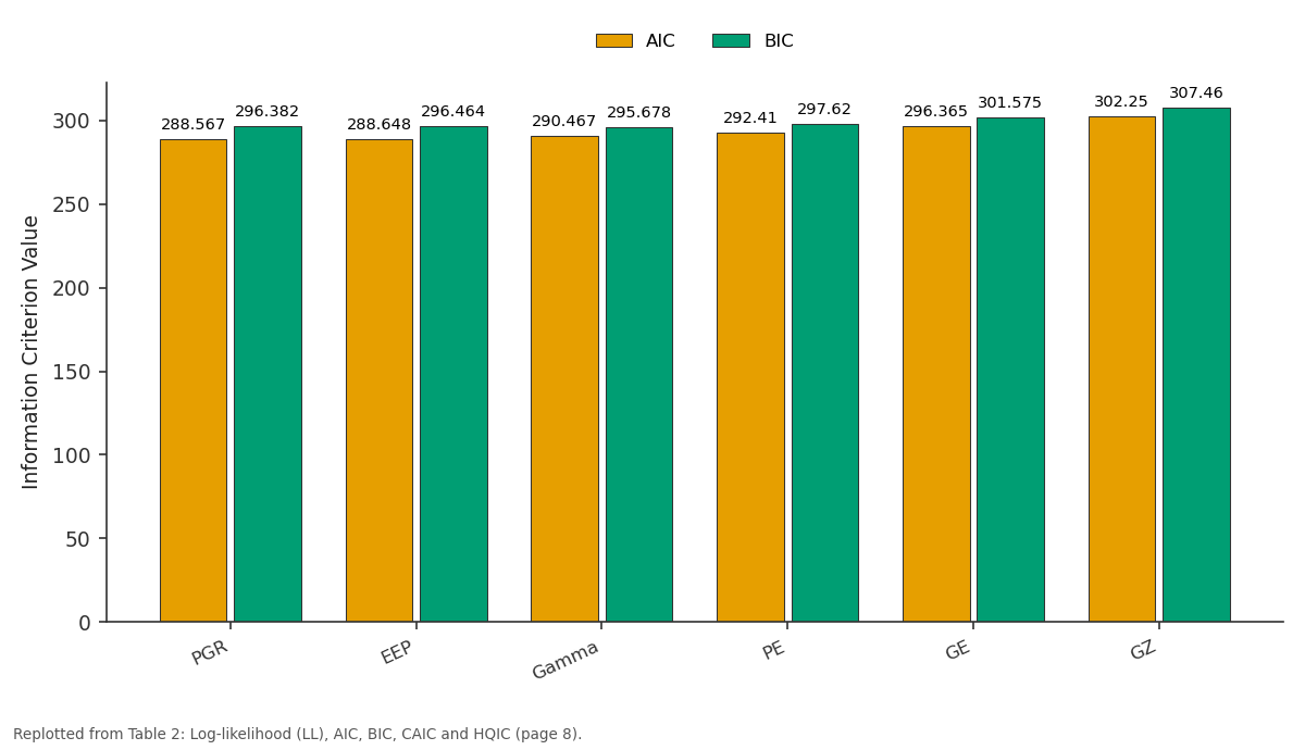
AIC and BIC: PGR vs EEP vs Gamma vs PE vs GE
Replotted from Table 2 (page 8) of the original paper. Every bar is the paper's own table value.
View source evidence ↗Figures & tables
From the original paper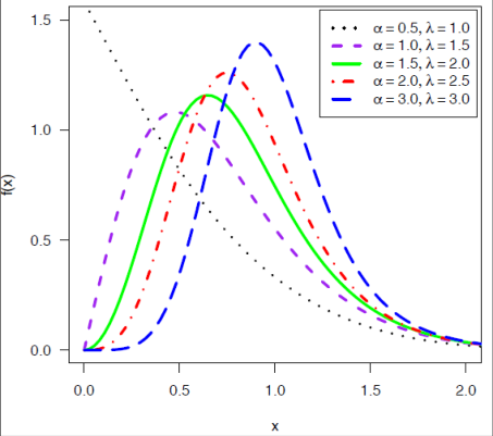 Figure 1
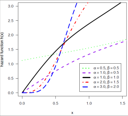 Figure 1
 Table 1
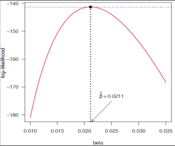 Figure 2
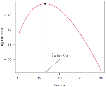 Figure 2
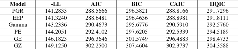 Table 2
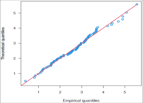 Figure 4
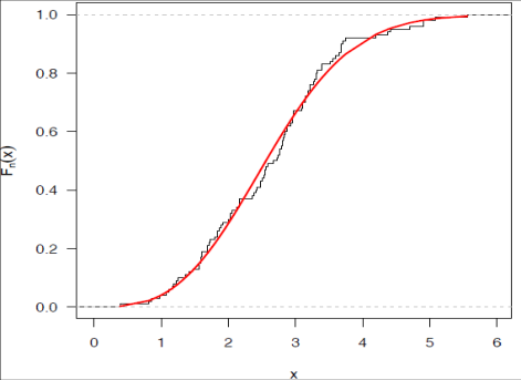 Figure 4
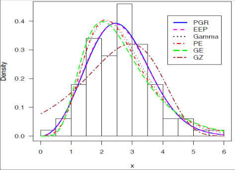 Figure 5
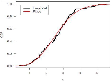 Figure 5
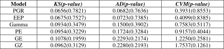 Table 3
Introduction
In the survival/reliability study, lifetime distributions are used to describe the length of the life of a component or device or a system. The lifetime distributions are most frequently used in the field like biological and medical sciences, engineering and manufacturing, etc. The exponential distribution is the most frequently used distribution due to the existence of simple elegant closed-form solutions to many survival analysis problems. The failure rate of the exponential distribution is constant but in real practice, the failure rates are not always constant. Hence in some situations, it seems to be inadequacy and unrealistic. For this, some modifications are needed to make exponential distribution more flexible. In recent, a new class of models has been introduced based on the modification of exponential distribution. Gupta and Kundu (1999) [6] introduced the generalized exponential (GE) distribution, this extended family can accommodate data with increasing and decreasing failure rate functions, Nadarajah and Kotz (2006) [24] have introduced a generalization referred to as the beta exponential distribution generated from the logit of a beta random variable. There are lots of lifetime models which are obtained by compounding with Zero truncated Poisson distribution some of them are as follows, A two-parameter exponential Poisson (EP) distribution has presented Kus (2007) [13] by modifying the exponential distribution with zero truncated Poisson distribution with a decreasing failure rate. The CDF of PE distribution is, ( ) ( )
While Barreto-Souza and Cribari-Neto (2009) [2] have introduced generalized EP distribution having the decreasing or increasing or upside-down bathtub shaped failure rate. This is the generalization of the distribution proposed by Kus (2007) [13] adding a power parameter to this distribution. Following a similar approach, Percontini et al. (2013) [18] have proposed the five-parameter beta Weibull Poisson distribution, which is obtained by compounding the Weibull Poisson and beta distributions. Following the same trend, Cancho (2011) [3] has developed a new distribution family also based on the exponential distribution with an increasing failure rate function known as Poisson exponential (PE) distribution. The cumulative distribution function of PE distribution can be expressed as
A two-parameter Poisson-exponential with increasing failure rate has been defined by (Louzada-Neto et al., 2011) [15] by using the same approach as used by (Cancho, 2011) [3] under the Bayesian approach. Alkarni and Oraby (2012) [1] have introduced a new lifetime family of distribution with a decreasing failure rate which is obtained by compounding truncated Poisson distribution and a lifetime model. The cumulative distribution function of the Poisson generating family is given by, ( )
Where the parameter is space and ( ) , Gy is the cumulative distribution function of any distribution. Using a parallel approach the Weibull power series class of distributions with Poisson has presented by (Morais & Barreto-Souza, 2011) [21] . Mahmoudi and Sepahdar (2013) [19] have defined a new four-parameter distribution with increasing, decreasing, bathtub-shaped, and unimodal failure rate called as the exponentiated Weibull-Poisson (EWP) distribution which has obtained by compounding exponentiated Weibull (EW) and Poisson distributions. Similarly, Lu and Shi (2012) have created the new compounding distribution named the Weibull-Poisson distribution having the shape of decreasing, increasing, upside-down bathtub-shaped, or unimodal failure rate function. Further Kaviayarasu and Fawaz (2017) [10] have made an extensive study on Weibull-Poisson distribution through a reliability sampling plan. Kyurkchiev et al. (2018) [14] has used the exponentiated exponential-Poisson as the software reliability model. Joshi & Kumar (2020) [9] has presented Poisson exponential power distribution and used different estimation methods to estimate the model parameter and hazard rate function can have increasing or j-shaped hazard rate. Chaudhary and Kumar (2020) [5] have presented the Poisson Inverse NHE distribution. Louzada et al. (2020) [16] has used different estimation methods to estimate the parameter of exponential-Poisson distribution using rainfall and aircraft data. The new Lindley-Rayleigh distribution has introduced by (Joshi & Kumar, 2020) [8] by compounding Rayleigh distribution with Lindley distribution. In this study, we propose a new distribution based on the generalized Rayleigh distribution has introduced by Surles and Padgett (2001) [30] introduced two-parameter Burr Type X distribution and correctly named as the generalized Rayleigh distribution for more detail see also (Surles and Padgett, 2004) [31] . Note that the two-parameter generalized Rayleigh distribution is a particular member of the exponentiated Weibull distribution, originally proposed by Mudholkar and Srivastava (1993) [22] . Kundu and Raqab (2005) [12] have presented the different estimation methods to estimate the unknown parameters of the generalized Rayleigh distribution. Chaudhary and Kumar (2020) [4] have presented the Logistic -Rayleigh distribution with increasing or j-shaped hazard rate function.
The CDF and PDF of the generalized Rayleigh distribution are respectively as
The main objective of this study is to develop a more flexible distribution by adding just one extra parameter to the generalized Rayleigh distribution to achieve a better fit to real data. The different sections of this study are arranged as follows; in Section 2 we present the new distribution Poisson generalized Rayleigh distribution (PGR) along with its mathematical and statistical properties. We widely discuss the maximum likelihood estimation method in Section 3. In Section 4 using a real dataset, we present the estimated values of the model parameters and their corresponding asymptotic confidence intervals and observed the Fisher information matrix. Besides, we have illustrated the different test criteria to assess the goodness of fit of the proposed model. Some concluding remarks are presented in Section 5.
The Poisson Generalized Rayleigh (PGR) Distribution
Alkarni and Oraby (2012) [1] have introduced a new lifetime class with a decreasing failure rate which is obtained by compounding zero truncated Poisson distribution and a lifetime distribution, where the compounding procedure follows the same way that was previously carried out by (Adamidis & Loukas, 1998). Let () Gx and () gx be the baseline cumulative distribution function and probability density function respectively then the Poisson family may be defined as, ( )
where ( ; ) Gx and ( ; , ) gx are the CDF and PDF of any baseline distribution the parameter space of the baseline distribution. Taking (1.4) and (1.5) as baseline distribution then (2.1) and (2.2) is reduced to the Poisson generalized Rayleigh (PGR) distribution can be defined as, Let X be a nonnegative random variable representing the lifetime of an item or component or a system in some population. The random variable X is said to follow the PGR distribution with parameters ( )
cumulative distribution function is given by ( ) ( )
And its corresponding probability density function is
Reliability function
The reliability function of PGR is denoted by ( ) R t , which is the probability of an item not failing up to time t, is defined by
. The survival /reliability function of the Poisson generalized Rayleigh distribution is given by ( ) ( )
The hazard rate function (HRF)
The hazard rate function for the PGR distribution can be defined as;
PGR then its hazard rate function is ( )
In Figure 1 we have demonstrated the graph for PDF and hazard function for PGR distribution for different values of the parameters. From Figure 1 (left panel), the density function of the PGR distribution can exhibit different shapes according to the values of the parameters. Figure 1 (right panel) demonstrates the increasing, decreasing, the j-shaped, and constant shape of the hazard rate.
The quantile function of PGR distribution
According to Hyndman and Fan (1996), the value of the p th quantile can be obtained by solving the following equation, ( ) ( )
And we get the quantile function by inverting CDF of PGR as
For the generation of the random numbers of the PGR distribution, we suppose simulating values of random variable X with the CDF (2.3). Let U denote a uniform random variable in (0, 1), then the simulated values of X can be obtained by
Median of PGR distribution
The median of X from the PGR distribution is simply obtained by replacing p = 0.5 in equation (2.7) which gives
Skewness and Kurtosis
The Bowley's measure of skewness based on quartiles was defined by (Kennedy & Keeping, 1962) [11] as,
and the coefficient of Moor's kurtosis measures based on octiles was defined by (Moors, 1988) [20] is given by
Methods of Estimation
The objective of estimation is to approximate the value of a model parameter based on sample information. The estimation theory deals with the basic problem of inferring some relevant features of a random experiment based on the observation of the experiment outcomes. There are so many methods for estimating unknown parameters of the model. We have considered the maximum likelihood estimation (MLE), method.
Maximum Likelihood Estimation (MLE) method
In this section, we have discussed the maximum likelihood estimators (MLE's) of the PGR (α, β, λ) distribution. Let ( ) 1 ,...,
be the observed values of size 'n' from PGR(α, β, λ), then the likelihood function for the parameter vector ( )
It is easy to deals with the log-likelihood function as, ( )
The elements of the score function ( ) ( )
The observed fisher information matrix ( ) Ô as an estimate of the information matrix ( )
Where H is the Hessian matrix. The Newton-Raphson algorithm to maximize the likelihood produces the observed information matrix. Therefore, the variancecovariance matrix is given by, ( )
var( ) cov( , ) ˆˆˆĉ ov( , ) cov( , ) var( )
Hence from the asymptotic normality of MLEs, approximate 100(1-α) % confidence intervals for α, β, and θ can be constructed as, /2 var( )
, where /2 Z is the upper percentile of standard normal variate.
Application with a real dataset
In this section, we have illustrated the applicability of PGR distribution using a real dataset used by previous researchers. The data gives 100 observations on breaking the stress of carbon fibers (in Gba) (Nichols & Padgett, 2006) [25] . The plots of profile log-likelihood function for the parameters α, β and λ have been displayed in Figure 2, and it is noticed that the ML estimates can be uniquely determined. The maximum likelihood estimates are calculated directly by using the optim() function in R software (R Core Team, 2020) [26] and (Rizzo, 2008) [28] by maximizing the likelihood function (3.1). We have obtained = 9.3340, = 0.3010, = 104.4248 and corresponding Log-Likelihood value is -141.2833. In Table 1 we have demonstrated the MLE's with their standard errors (SE) and 95% confidence interval for α, β, and . To judge the goodness-of-fit of the Poisson generalized Rayleigh distribution, we have considered some well-known distribution for comparison purpose which are listed below,
| Parameter | MLE | SE | 95% ACI |
|---|---|---|---|
| alpha | 1.5466 | 0.1492 | (1.2542, 1.8389) |
| beta | 0.0211 | 0.0053 | (0.0106, 0.0315) |
| lambda | 16.4523 | 2.9579 | (10.6548, 22.2498) |
Table text extracted from the original PDF; superscript letters are shown inline. The original table image is below.
View original table image
Exponentiated Exponential Poisson (EEP)
The probability density function of EEP (Ristić & Nadarajah, 2014) [27] can be expressed as
Gamma distribution
The density of Gamma distribution with parameters and is ( )
Poisson-exponential distribution (PE)
The probability density function of Poisson-exponential (PE) distribution was defined by (Louzada-Neto et al., 2011) [15] also it was used by (Rodrigues et al., 2018) [29] is
Generalized Exponential (GE) distribution
The probability density function of generalized exponential distribution (Gupta & Kundu, 1999) [6] can be written as
Gompertz distribution (GZ)
The probability density function of Gompertz distribution (Murthy et al., 2003) [23] with parameters α and θ is ( ) ( )
To assess the goodness of fit of a given distribution we generally use the PDF and CDF plot. To get the additional information we have to plot Q-Q and KS plots. In particular, the Q-Q plot may provide information about the lack-of-fit at the tails of the distribution, whereas the KS plot emphasizes the lack-of-fit. From Figure 4 it is verified that the PGR model fits the data very well. 4. The Histogram and the density function of fitted distributions and Empirical distribution function with the estimated distribution function of PGR and some selected distributions are presented in Figure 5. To compare the goodness-of-fit of the PGR distribution with other competing distributions we have presented the value of Kolmogorov-Simnorov (KS), the Anderson-Darling (AD) and the Cramer-Von Mises (CVM) statistics in Table 5. It is observed that the PGR distribution has the minimum value of the test statistic and higher p-value thus we conclude that the PGR distribution gets quite better fit and more consistent and reliable results from others taken for comparison.
Conclusion
In this study, we have studied the three-parameter Poisson generalized Rayleigh distribution. For our study, we provided the probability density function, the cumulative distribution function, and the shapes of the hazard rate function. The shape of the PDF of the PGR distribution is unimodal and positively skewed, while the hazard function of the PGR distribution is increasing, decreasing, and the j-shaped and constant shape of the hazard rate. The P-P and Q-Q plots showed that the purposed distribution is quite better for fitting the real dataset. Finally, using a real data set we have explored some well-known estimation methods namely the maximum likelihood estimation (MLE) method. Further, we also construct the asymptotic confidence interval for MLEs. The application illustrates that the proposed model provides a consistently better fit than other underling models. We expect that this model will contribute to the field of survival analysis.
Figures and tables from the paper
| Model | -LL | AIC | BIC | CAIC | HQIC |
|---|---|---|---|---|---|
| PGR | 141.2833 | 288.5666 | 296.3821 | 288.8166 | 291.7296 |
| EEP | 141.3240 | 288.6481 | 296.4636 | 288.8981 | 291.8111 |
| Gamma | 143.2336 | 290.4673 | 295.6776 | 290.5910 | 292.5760 |
| PE | 144.2051 | 292.4102 | 297.6205 | 292.5339 | 294.5189 |
| GE | 146.1823 | 296.3646 | 301.5749 | 296.4883 | 298.4733 |
| GZ | 149.1250 | 302.2500 | 307.4604 | 302.3737 | 304.3588 |
Table text extracted from the original PDF; superscript letters are shown inline. The original table image is below.
View original table image
| Model | KS(p-value) | AD(p-value) | CVM(p-value) |
|---|---|---|---|
| PGR | 0.0656(0.7821) | 0.0682(0.7636) | 0.3931(0.8553) |
| EEP | 0.0675(0.7527) | 0.0723(0.7385) | 0.4099(0.8385) |
| Gamma | 0.0934(0.3479) | 0.1500(0.3902) | 0.7583(0.5117) |
| PE | 0.0954(0.3229) | 0.1724(0.3284) | 0.9157(0.4044) |
| GE | 0.1078(0.1959) | 0.2293(0.2174) | 1.2250(0.2581) |
| GZ | 0.0962(0.3129) | 0.2280(0.2193) | 1.7537(0.1261) |
Table text extracted from the original PDF; superscript letters are shown inline. The original table image is below.
View original table image
References
31 in the original paper- Alkarni S, Oraby A. A compound class of Poisson and lifetime distributions, J Stat. Appl. Pro 2012;1(1):45-51.
- Barreto-Souza W, Cribari-Neto F. A generalization of the exponential-Poisson distribution. Statistics and Probability Letters 2009;79:2493-2500.
- Cancho VG, Louzada-Neto F, Barriga GDC. The Poisson-exponential lifetime distribution. Computational Statistics and Data Analysis 2011;55:677-686.
- Chaudhary AK, Kumar V. The Logistic -Rayleigh Distribution with Properties and Applications. International Journal of Statistics and Applied Mathematics 2020;5(6):12-19.
- Chaudhary AK, Kumar V. Poisson Inverse NHE Distribution with Theory and Applications. International Journal of Science and Research (IJSR) 2020;9(12):1603-1610.
- Gupta RD, Kundu D. Theory & methods: Generalized exponential distributions. Australian & New Zealand Journal of Statistics 1999;41(2):173-188.
- Hyndman RJ, Fan Y. Sample quantiles in statistical packages. The American Statistician 1996;50(4):361-365.
- Joshi RK, Kumar V. New Lindley-Rayleigh Distribution with Statistical properties and Applications. International Journal of Mathematics Trends and Technology (IJMTT) 2020;66(9):197-208.
- Joshi RK, Kumar V. Poisson Exponential Power distribution: Properties and Application. International Journal of Mathematics & Computer Research 2020;8(11):2152-2158.
- Kaviayarasu V, Fawaz P. A Reliability Sampling Plan to ensure Percentiles through Weibull Poisson Distribution, International Journal of Pure and Applied Mathematics 2017;117(13):155-163.
- Kenney JF, Keeping. E.S. Mathematics of Statistics. (3 rd ed.). Chapman & Hall Ltd, New Jersey 1962.
- Kundu D, Raqab MZ. Generalized Rayleigh distribution: different methods of estimations. Computational statistics & data analysis 2005;49(1):187-200.
- Kus C. A new lifetime distribution. Computational Statistics and Data Analysis 2007;51:4497-4509.
- Kyurkchiev VESSELIN, Kiskinov HRISTO, Rahneva OLGA, Spasov GEORGI. A Note on the Exponentiated ExponentialPoisson Software Reliability Model. Neural, Parallel, and Scientific Computations 2018;26(3):257-267.
- Louzada-Neto F, Cancho VG, Barriga GDC. The Poisson-exponential distribution: A Bayesian approach, Journal of Applied Statistics 2011;38(6):1239-1248.
- Louzada F, Luiz Ramos P, Henrique Ferreira P. Exponential-Poisson distribution: estimation and applications to rainfall and aircraft data with zero occurrences. Communications in Statistics-Simulation and Computation 2020;49(4):1024-1043.
- Lu W, Shi D. A new compounding life distribution: the Weibull-Poisson distribution, Journal of Applied Statistics 2012;39(1):21-38.
- Percontini A, Blas B, Cordeiro GM. The beta weibull Poisson distribution. Chilean journal of Statistics 2013;4(2):3-26.
- Mahmoudi E, Sepahdar A. Exponentiated Weibull-Poisson distribution: Model, properties and applications. Mathematics and computers in simulation 2013;92:76-97.
- Moors JJA. A quantile alternative for kurtosis. Journal of the Royal Statistical Society: Series D (The Statistician) 1988;37(1):25-32.
- Morais A, Barreto-Souza W. A compound class of Weibull and power series distributions. Computational Statistics and Data Analysis 2011;55:1410-1425.
- Mudholkar GS, Srivastava DK. Exponentiated Weibull family for analyzing bathtub failure data. IEEE Trans. Reliability 1993;42:299-302.
- Murthy DNP, Xie M, Jiang R. Weibull Models, Wiley, New York 2003.
- Nadarajah S, Kotz S. The beta exponential distribution. Reliability engineering & system safety 2006;91(6):689-697.
- Nichols MD, Padgett WJ. A bootstrap control chart for Weibull percentiles. Quality and reliability engineering international 2006;22(2):141-151.
- Core Team R. R: A language and environment for statistical computing. R Foundation for Statistical Computing, Vienna, Austria 2020. URL https://www.R-project.org/.
- Ristić MM, Nadarajah S. A new lifetime distribution. Journal of Statistical Computation and Simulation 2014;84(1):135-150.
- Rizzo ML. Statistical computing with R. Chapman & Hall/CRC 2008.
- Rodrigues GC, Louzada F, Ramos PL. Poisson-exponential distribution: different methods of estimation, Journal of Applied Statistics 2018;45(1):128-144.
- Surles JG, Padgett WJ. Inference for reliability and stress-strength for a scaled Burr Type X distribution. Lifetime Data Analysis 2001;7(2):187-200.
- Surles JG, Padgett WJ. Some properties of a scaled Burr type X distribution. Journal of statistical planning and inference 2005;128(1):271-280.
Cited by 3
From OpenAlex, OpenCitations and reference lists read by Scinovex
- Control Charts for Overdispersed Count Data: Exploring the Poisson Chris‐Jerry Distribution in Agriculture and Medicine ↗
Tabassum Naz Sindhu, Anum Shafiq, Abdon Atangana, Tahani Abdulrahmaan Abushal, Alia A. Alkhathami · Quality and Reliability Engineering International · 2025
ABSTRACT Statistical process control (SPC) is vital for overseeing processes and ensuring quality standards, with control charts being key tools in this process. As manufacturing systems and components become more complex, there is an increasing demand for control charts built on advanced statistical distributions. The Poisson‐based count chart is commonly used to monitor nonconformities in production, but its use depends…
❝ 6 - HALF CAUCHY GENERALIZED RAYLEIGH DISTRIBUTION: THEORY AND APPLICATION ↗
Laxmi Prasad Sapkota, Vijay Kumar · South East Asian J of Mathematics and Mathematical Sciences · 2023
We develop a new three parameter distribution using the half-Cauchy family of distributions, called the half-Cauchy generalized Rayleigh distribution. Some statistical properties and characteristics of the proposed distribution are provided and obtained, including the explicit expressions for the survival function, median, hazard function, mode, moments, mean deviation, order statistics, cumulative hazard function, quantiles, and the measures of dispersion based on…
❝ 3PDF - NeuDist: Univariate Continuous Distributions with Model Diagnostics ↗
Vijay Kumar, Laxmi Prasad Sapkota, Pankaj Kumar, Lal Babu Sah Telee · 2026
Implements univariate continuous probability distributions and associated model diagnostics based on the Lindley, Logistic, Half-Cauchy, Half-Logistic, and Poisson families. Provides functions for probability density, cumulative distribution, quantile, and hazard evaluation, random variate generation, and diagnostic procedures including Q-Q and P-P plots, goodness-of-fit tests, and model selection criteria.
❝ 2PDF