
Research article · 2016 · Full text
International Journal of Statistics and Applied MathematicsImplementing Chiu’s fixed lifetime inventory model
Volume 1(5) · Pages 06–13
Research areasSupply Chain and Inventory ManagementReliability and Maintenance OptimizationAdvanced Statistical Process Monitoring
Abstract
Author-writtenThe fixed lifetime inventory system with zero or positive leadtime has being considered by various authors, with the aim of reducing the quantity outdating in the inventory system. Chiu (1995), considered the positive leadtime case by approximating the expected shortage quantity, the expected outdate quantity and the expected on hand inventory. His result was a Q, R ordering policy where Q and r are the ordered quantity and the reorder point respectively. In this work, we examine Chiu’s implementation of the model, use simple minimization method to obtain the order quantity and modify the total cost function obtained by Chiu. Also, we consider the case where the reorder point is not zero, which Chiu did not considered.
Summary
Source-checkedPlain-language reading of the full paper, prepared with AI and checked against the text. Each point links to the authors' own words.
Why it matters
- Fixed lifetime products, such as drugs, blood, and foodstuffs, have a predefined shelf life and expiration dates. View evidence ↗
- Inventory of these products is reduced by either customer demand or outdating, which happens when a product expires before it can be used. View evidence ↗
- Research into fixed lifetime inventory systems aims to minimize the amount of product that expires (outdates) while accounting for lead times. View evidence ↗
The question
- The study aims to implement Chiu's inventory model using a simple minimization method, modify the total cost function, and analyze cases where the reorder point is non-zero. View evidence ↗
What they did
- The authors implemented the model by calculating partial derivatives of the cost function with respect to the order quantity using Mathematical 8 software. View evidence ↗
- The minimization method's results for order quantity (Qm) were compared against Chiu's algorithm (Qc) using constant values of c=1, h=1, and d=1. View evidence ↗
- The authors modified the cost function because they found Chiu's outdate quantity calculation misleading regarding lead time demand and the timing of outdating. View evidence ↗
- To determine both order quantity (Q) and reorder point (r), the authors first assumed r=0 to find Q, then used that Q to solve for r. View evidence ↗
What they found
- The modified model generally resulted in lower total costs than Chiu's model because it produced lower outdate quantities. View evidence ↗
- A negative outdate quantity in the model indicates that no products expired, but shortages occurred instead. View evidence ↗
- For a non-zero reorder point r=10 with parameters w=1, m=5, k=1, the order quantity Q was found to be 0.3108. View evidence ↗
What it means
- The authors conclude that using a simple minimization method allows Chiu's model to be solved, reducing the uncertainty of the original algorithm. View evidence ↗
- The authors recommend the redefined cost function as it generally results in lower total costs due to reduced outdate quantities. View evidence ↗
Visual summary
3 visualsIllustrations explain the paper; charts are replotted from the paper's own table values.

Inventory Depletion Process
AI-generated conceptual illustration (Cardboard boxes of perishable pharmaceutical vials on a warehouse shelf). It explains the idea and does not show study data.
View source evidence ↗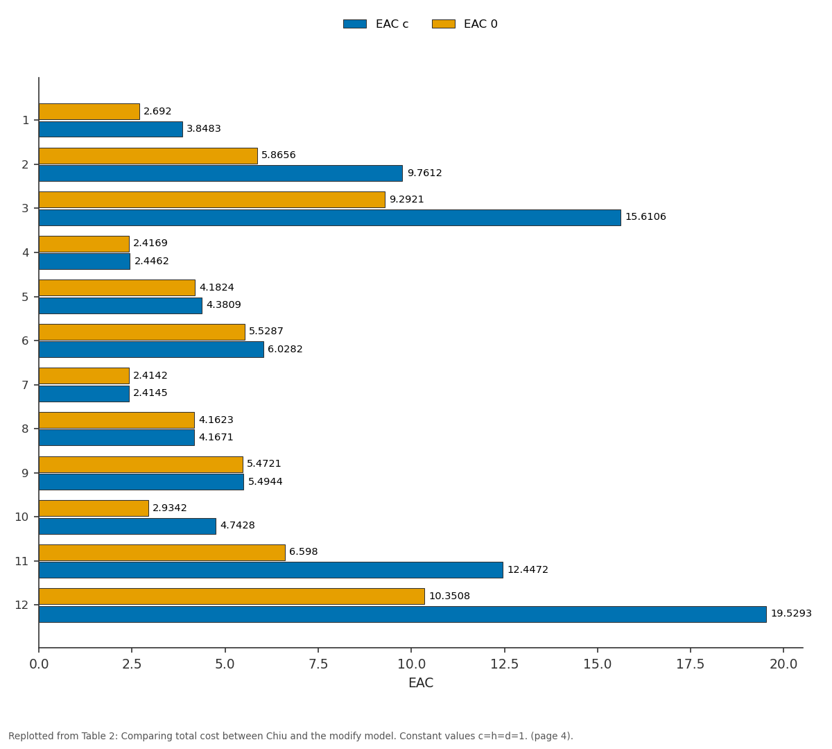
EAC c and EAC 0: 1 vs 2 vs 3 vs 4 vs 5
Replotted from Table 2 (page 4) of the original paper. Every bar is the paper's own table value.
View source evidence ↗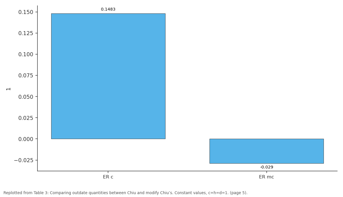
1: ER c vs ER mc
Replotted from Table 3 (page 5) of the original paper. Every bar is the paper's own table value.
View source evidence ↗Figures & tables
From the original paper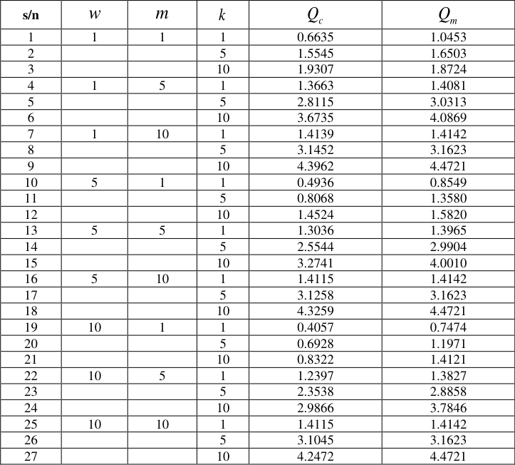 Table 1
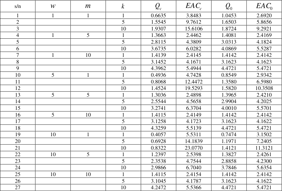 Table 2
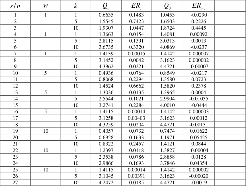 Table 3
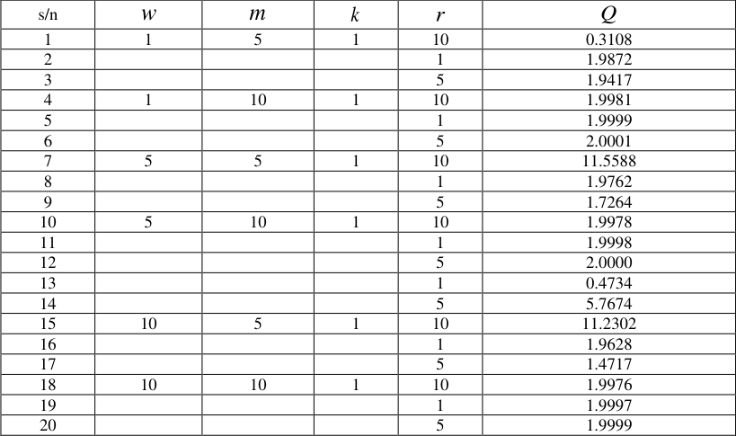 Table 4
Introduction
Many researchers have worked on the fixed lifetime inventory system. Schmidt and Nahmias (1985) [3] , Liu and Lian (1999) [5] , Omosigho (2002) [4] , Olsson and Tydesjo (2010) [6] , Shen et al. (2012) [7] to mention a few. All of these authors worked on reducing the amount of items outdating in a fixed lifetime inventory system. Fixed lifetime products are products with a predefined shelf life and normally carry expiration dates on them. While in inventory, these products are depleted by either demand or outdating. Outdating occur when a product is not used to meet demand by the end of its useful lifetime in inventory. Examples of such products include foodstuffs, drugs, blood, batteries etc. This work examine Chiu's model on fixed lifetime, redefine the outdate quantity and consider the case where the reorder point is not zero. Chiu (1995), considered the case of an approximation to the continuous review inventory model with perishable items and positive lead time and came up with the total cost function
In order to search for a minimum Chiu took the partial derivatives of (1) with respect to Q and r, setting each to zero, and obtained
Equations ( 2) and (3) could not be solved explicitly, so he developed a solution algorithm to solve the equations for Q and r. However, Chiu reported that, " it requires an extremely large number of iterations to complete the steps of the solution algorithm and the intolerably computational efforts makes it impossible to obtain a convergent solution". The result for this model is of the form (Q, r) where Q is ordered whenever on hand inventory drops to r, which imply that the decision to reorder depends on the quantity of products on hand. Furthermore, Chiu obtained numerical results for the case where the reorder point is zero. To implement the model, we obtain the partial derivatives of equation (1) with respect to the ordered quantity using Mathematical 8, equate to zero and solve the resulting equation.
Going forward, we take f (inf inity) to be zero and consider the cases where 0 0 r and r which was not considered by Chiu.
Case 1. assume r=0 and simplifying, we have
We solved equation ( 4) using mathematical 8 and the results obtained for the ordered quantity is compared with the results obtained by Chiu and shown in table1 For the total cost function, we observe that the outdate quantity obtained by Chiu, shown below
| s/n | w | m | k | Q c | Q m |
|---|---|---|---|---|---|
| 1 | 1 | 1 | 1 | 0.6635 | 1.0453 |
| 2 | 5 | 1.5545 | 1.6503 | ||
| 3 | 10 | 1.9307 | 1.8724 | ||
| 4 | 1 | 5 | 1 | 1.3663 | 1.4081 |
| 5 | 5 | 2.8115 | 3.0313 | ||
| 6 | 10 | 3.6735 | 4.0869 | ||
| 7 | 1 | 10 | 1 | 1.4139 | 1.4142 |
| 8 | 5 | 3.1452 | 3.1623 | ||
| 9 | 10 | 4.3962 | 4.4721 | ||
| 10 | 5 | 1 | 1 | 0.4936 | 0.8549 |
| 11 | 5 | 0.8068 | 1.3580 | ||
| 12 | 10 | 1.4524 | 1.5820 | ||
| 13 | 5 | 5 | 1 | 1.3036 | 1.3965 |
| 14 | 5 | 2.5544 | 2.9904 | ||
| 15 | 10 | 3.2741 | 4.0010 | ||
| 16 | 5 | 10 | 1 | 1.4115 | 1.4142 |
| 17 | 5 | 3.1258 | 3.1623 | ||
| 18 | 10 | 4.3259 | 4.4721 | ||
| 19 | 10 | 1 | 1 | 0.4057 | 0.7474 |
| 20 | 5 | 0.6928 | 1.1971 | ||
| 21 | 10 | 0.8322 | 1.4121 | ||
| 22 | 10 | 5 | 1 | 1.2397 | 1.3827 |
| 23 | 5 | 2.3538 | 2.8858 | ||
| 24 | 10 | 2.9866 | 3.7846 | ||
| 25 | 10 | 10 | 1 | 1.4115 | 1.4142 |
| 26 | 5 | 3.1045 | 3.1623 | ||
| 27 | 10 | 4.2472 | 4.4721 |
Table text extracted from the original PDF; superscript letters are shown inline. The original table image is below.
View original table image
Is misleading for the following reasons (1) r is designed to satisfy the leadtime demand and not demand during M+L units of time as giving in the second term of the outdate quantity (2) The first term calculates the outdate quantities for both the previous and current orders. We believe that outdate quantity should be a function of previous order only, since the issuing policy is oldest unit first.
We this, the outdate quantity should be
We compare the total cost using equations ( 1) and ( 5) for the values of Q obtained in table 1. When the outdate quantity is negative, it imply that no outdating occur from that order, but there will be shortages.
Simplifying equation ( 6) we have
Expanding and further simplifying gives equation ( 8) and ( 9)
We use mathematical 8 to solve equation (9), table4 shows values of Q obtained for some values of r. Where there are no past records to determine the value of r, we differentiate (1) with respect to the reorder point and obtain an equation for the reorder point. r
| s/n | w | m | k | r | Q |
|---|---|---|---|---|---|
| 1 | 1 | 5 | 1 | 10 | 0.3108 |
| 2 | 1 | 1.9872 | |||
| 3 | 5 | 1.9417 | |||
| 4 | 1 | 10 | 1 | 10 | 1.9981 |
| 5 | 1 | 1.9999 | |||
| 6 | 5 | 2.0001 | |||
| 7 | 5 | 5 | 1 | 10 | 11.5588 |
| 8 | 1 | 1.9762 | |||
| 9 | 5 | 1.7264 | |||
| 10 | 5 | 10 | 1 | 10 | 1.9978 |
| 11 | 1 | 1.9998 | |||
| 12 | 5 | 2.0000 | |||
| 13 | 1 | 0.4734 | |||
| 14 | 5 | 5.7674 | |||
| 15 | 10 | 5 | 1 | 10 | 11.2302 |
| 16 | 1 | 1.9628 | |||
| 17 | 5 | 1.4717 | |||
| 18 | 10 | 10 | 1 | 10 | 1.9976 |
| 19 | 1 | 1.9997 | |||
| 20 | 5 | 1.9999 |
Table text extracted from the original PDF; superscript letters are shown inline. The original table image is below.
View original table image
We can use equations ( 9) and ( 12) to obtain values of Q and r 1. First assume r =0 and use (9) to obtain Q.
2. The value of Q obtained is then used in (12) to obtain the value of r.
Observe that for the minimization problem, the resulting polynomial have a number of roots. Deciding which of the roots is the order quantity, we follow the steps below.
Step 1: Eliminate all the complex roots, as the order quantity cannot be represented by a Complex number, but by a real number.
Step 2: Eliminate all negative roots, since the order quantity cannot be a negative number.
Step 3: When there is only one positive root, its taken as the value.
Step 4: If there are more than one positive root, we pick the minimum of the positive roots as our order quantity, since higher values may increase the outdating quantity.
Step 5: If zero is the only non-negative and non-complex root of the polynomial, we use the aspiration Level criterion to determine the order quantity. The aspiration level is the degree/level of Performance (determined by past experience) that a firm desires to attain or feel it can achieve. For details on aspiration level criterion see Vahid et al. (1992).
Conclusion
With simple minimization, the model obtained by Chiu can be solved. This will reduce the uncertainty associated with Chiu's algorithm. The results obtained using the modify method, shows that the total cost for the model is generally lower for the redefined form when compared with results obtained by Chiu, the reason for this is because the outdate quantities are lower for the redefined form. The ordered quantities when 0 r were also obtained for some values of r.
Figures and tables from the paper
| s/n | w | m | k | Q c | EAC c | Q 0 | EAC 0 |
|---|---|---|---|---|---|---|---|
| 1 | 1 | 1 | 1 | 0.6635 | 3.8483 | 1.0453 | 2.6920 |
| 2 | 5 | 1.5545 | 9.7612 | 1.6503 | 5.8656 | ||
| 3 | 10 | 1.9307 | 15.6106 | 1.8724 | 9.2921 | ||
| 4 | 1 | 5 | 1 | 1.3663 | 2.4462 | 1.4081 | 2.4169 |
| 5 | 5 | 2.8115 | 4.3809 | 3.0313 | 4.1824 | ||
| 6 | 10 | 3.6735 | 6.0282 | 4.0869 | 5.5287 | ||
| 7 | 1 | 10 | 1 | 1.4139 | 2.4145 | 1.4142 | 2.4142 |
| 8 | 5 | 3.1452 | 4.1671 | 3.1623 | 4.1623 | ||
| 9 | 10 | 4.3962 | 5.4944 | 4.4721 | 5.4721 | ||
| 10 | 5 | 1 | 1 | 0.4936 | 4.7428 | 0.8549 | 2.9342 |
| 11 | 5 | 0.8068 | 12.4472 | 1.3580 | 6.5980 | ||
| 12 | 10 | 1.4524 | 19.5293 | 1.5820 | 10.3508 | ||
| 13 | 5 | 5 | 1 | 1.3036 | 2.4898 | 1.3965 | 2.4210 |
| 14 | 5 | 2.5544 | 4.5658 | 2.9904 | 4.2025 | ||
| 15 | 10 | 3.2741 | 6.3704 | 4.0010 | 5.5701 | ||
| 16 | 5 | 10 | 1 | 1.4115 | 2.4149 | 1.4142 | 2.4142 |
| 17 | 5 | 3.1258 | 4.1723 | 3.1623 | 4.1622 | ||
| 18 | 10 | 4.3259 | 5.5139 | 4.4721 | 5.4721 | ||
| 19 | 10 | 1 | 1 | 0.4057 | 5.5311 | 0.7474 | 3.1502 |
| 20 | 5 | 0.6928 | 14.1839 | 1.1971 | 7.2405 | ||
| 21 | 10 | 0.8322 | 23.0770 | 1.4121 | 11.3121 | ||
| 22 | 10 | 5 | 1 | 1.2397 | 2.5398 | 1.3827 | 2.4261 |
| 23 | 5 | 2.3538 | 4.7544 | 2.8858 | 4.2300 | ||
| 24 | 10 | 2.9866 | 6.7040 | 3.7846 | 5.6354 | ||
| 25 | 10 | 10 | 1 | 1.4115 | 2.4154 | 1.4142 | 2.4142 |
| 26 | 5 | 3.1045 | 4.1787 | 3.1623 | 4.1622 | ||
| 27 | 10 | 4.2472 | 5.5366 | 4.4721 | 5.4721 |
Table text extracted from the original PDF; superscript letters are shown inline. The original table image is below.
View original table image
| s /n | w | k | Q c | ER c | Q 0 | ER mc | — |
|---|---|---|---|---|---|---|---|
| 1 | 1 | 1 | 0.6635 | 0.1483 | 1.0453 | -0.0290 | |
| 2 | 5 | 1.5545 | 0.7423 | 1.6503 | 0.2226 | ||
| 3 | 10 | 1.9307 | 1.0447 | 1.8724 | 0.4445 | ||
| 4 | 1 | 1 | 1.3663 | 0.0154 | 1.4081 | 0.00092 | |
| 5 | 5 | 2.8115 | 0.1391 | 3.0313 | 0.0013 | ||
| 6 | 10 | 3.6735 | 0.3320 | 4.0869 | -0.0237 | ||
| 7 | 1 | 1 | 1.4139 | 0.00015 | 1.4142 | 0.000007 | |
| 8 | 5 | 3.1452 | 0.0042 | 3.1623 | 0.000002 | ||
| 9 | 10 | 4.3962 | 0.0221 | 4.4721 | -0.00007 | ||
| 10 | 5 | 1 | 0.4936 | 0.0764 | 0.8549 | -0.0217 | |
| 11 | 5 | 0.8068 | 0.2294 | 1.3580 | 0.0723 | ||
| 12 | 10 | 1.4524 | 0.6662 | 1.5820 | 0.2378 | ||
| 13 | 5 | 1 | 1.3036 | 0.0135 | 1.3965 | 0.0004 | |
| 14 | 5 | 2.5544 | 0.1021 | 2.9904 | -0.01035 | ||
| 15 | 10 | 3.2741 | 0.2284 | 4.0010 | -0.0444 | ||
| 16 | 5 | 1 | 1.4115 | 0.00014 | 1.4142 | 0.000003 | |
| 17 | 5 | 3.1258 | 0.00403 | 3.1623 | 0.00012 | ||
| 18 | 10 | 4.3259 | 0.0204 | 4.4721 | -0.00131 | ||
| 19 | 10 | 1 | 0.4057 | 0.0732 | 0.7474 | 0.01622 | |
| 20 | 5 | 0.6928 | 0.1633 | 1.1971 | 0.05425 | ||
| 21 | 10 | 0.8322 | 0.2457 | 1.4121 | 0.0844 | ||
| 22 | 10 | 1 | 1.2397 | 0.0118 | 1.3827 | -0.00004 | |
| 23 | 5 | 2.3538 | 0.0786 | 2.8858 | 0.0128 | ||
| 24 | 10 | 2.9866 | 0.1693 | 3.7846 | 0.04354 | ||
| 25 | 10 | 1 | 1.4115 | 0.00014 | 1.4142 | 0.000002 | |
| 26 | 5 | 3.1045 | 0.00391 | 3.1623 | -0.00020 | ||
| 27 | 10 | 4.2472 | 0.0185 | 4.4721 | -0.0019 |
Table text extracted from the original PDF; superscript letters are shown inline. The original table image is below.
View original table image
References
7 in the original paper- Chiu HN. An approximation to the continuous review inventory model with perishable items and lead times. European journal of operational research 1995;87:93-108.
- Vahid et al. An aspiration level interactive model for multiple criteria decision marking. Journal of Computers Operations Research 1992;19(7):671-681.
- Schmidt CP, Nahmias S. (S-1, S) Policies for Perishable Inventory. Management Science 1985;31(6):719-728.
- Omosigho SE. Determination of Outdate and Shortage Quantities in the Inventory Problem with fixed Lifetime. International Journal Computer Math 2002;79(11):1169-1177.
- Liu L, Lian Z. (s,S) Continuous Review Models for Products with Fixed Lifetime. Operations Research 1999;47(1):150-158.
- Olsson F, Tydesjo P. Inventory Problems with Perishable items: Fixed Lifetimes and Backlogging. European Journal of Operational Research 2010:202:131-137.
- Shen Z, Dessouky M, Ordonez F. Perishable inventory management system with a minimum volume constraint. Journal of the Operational Research Society 2011;62:2063-2082.