
Research article · 2020 · Full text
International Journal of Statistics and Applied MathematicsInformation-based stochastic volatility model using the extended Kalman filter
Volume 5(5) · Pages 124–127
Research areasComplex Systems and Time Series AnalysisStochastic processes and financial applicationsFinancial Risk and Volatility Modeling
Abstract
Author-writtenThis study explores the use of non-linear filtering in an information-based stochastic volatility model. The stochastic differential equations in the model incorporate information which is the sum of true information about the future cash flows and noise which distorts the true information. It is assumed that there exists a market information process consisting of a combination of these two sources of information. The volatility process in the model is non-linear and gaussian which makes the use of the extended Kalman filter approach ideal. The study first obtains a state space model and the extended Kalman filter is then used to model volatility based on it. The modelled volatility is used to determine the extent to which the price of the information-based stochastic volatility model is affected by fluctuations in volatility. Using simulated data, the study finds that there’s a general increase in volatility as the price obtained from the model increases.
Summary
Source-checkedPlain-language reading of the full paper, prepared with AI and checked against the text. Each point links to the authors' own words.
Why it matters
- The Black Scholes model assumes constant volatility, but this assumption is considered non-ideal by various researchers. View evidence ↗
- Stochastic volatility models (SVM) are used to address the 'volatility smile,' which the Black Scholes model fails to detect because volatility varies over time. View evidence ↗
- The information-based pricing framework improves upon other SVMs because volatility is naturally stochastic based on market information rather than being pre-specified. View evidence ↗
The question
- The study aims to use the extended Kalman filter (EKF), a non-linear filtering approach, to model volatility within an information-based stochastic volatility model (ISVM). View evidence ↗
What they did
- The researchers first developed a state space model, which then served as the basis for modeling volatility using the EKF. View evidence ↗
- The model used constant estimated values of 0.5 for vk-1, 0.2 for κk-1, and 0.1 for the interest rate r. View evidence ↗
- The simulation initialized the state process (x̂k-1) at 0 and the posterior state estimate error covariance (P0) at 1. View evidence ↗
- The measurement process observations representing price were obtained via simulation using standard normally distributed errors with R ~ N(0, 0.01). View evidence ↗
What they found
- Analysis of simulated data revealed that volatility generally increases as the price derived from the model increases. View evidence ↗
- The results of the EKF application showed that estimated volatility generally increases in correlation with price increases. View evidence ↗
What it means
- The authors conclude that the EKF is a practical technique for modeling volatility because its iterative update steps align with the fact that current volatility depends on previous volatility. View evidence ↗
- The authors note that the interest rate was assumed to be constant and recommend future research where the interest rate is treated as stochastic. View evidence ↗
- The authors suggest comparing EKF results with other non-linear filtering techniques, such as particle filtering or the unscented Kalman filter, to find the most suitable method for ISVM volatility modeling. View evidence ↗
Visual summary
1 visualsIllustrations explain the paper; they do not show study data.

EKF Volatility Modeling Workflow
AI-generated conceptual illustration (A digital signal processing circuit board with a central microprocessor and oscillating wave patterns). It explains the idea and does not show study data.
View source evidence ↗Figures & tables
From the original paper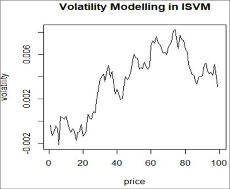 Figure 1
Introduction
Following the collapse of the stock market in the late 1980's as documented in (Bernhardt & Eckblad, 2013) [1] , there has been significant research on the volatility of option prices. The Black Scholes model as presented in (Black & Scholes, 1973) [7] makes the assumption that volatility is constant. This assumption has been shown by various authors not to be ideal despite the model being used successfully in pricing options (Bernhardt & Eckblad, 2013) [1] , (Javaheri, 2005) [12] , (Pottinton, 2017) [13] and (Bergomi, 2004) [14] . Models which make an assumption that the volatility is stochastic are known as stochastic volatility models (SVM). These models can be used to address the failure of the Black Scholes model to detect the volatility smile which arises due to the variation of volatility with time as suggested by (Javaheri, 2005) [12] . The Heston model as presented by S. Heston in (Heston, 1993) is a popular SVM which is used in pricing options. The variance process in the model is assumed to follow a Cox Ingersoll Ross (CIR) process, (Cox et al.,1985) [10] . Despite the fact that the Heston model is an improvement to the Black Scholes model, it suffers from the weakness that the volatility dynamics are pre-specified which shows an adhoc nature. The information based pricing framework by Brody, Hughson and Macrina, (Macrina, 2006) [3] tends to be an improvement to this as the volatility dynamics are not prespecified. The volatility is shown to be naturally stochastic as a result of the assumed market information process. A non-linear filtering approach, in particular the extended Kalman filter (EKF) is used in this study to model volatility from an information-based stochastic volatility model (ISVM). The ISVM is derived from the information based pricing framework outlined in (Macrina, 2006) [3] . Javeheri et al. demonstrate the application of non-linear filtering to the Heston Model, (Javaheri et al., 2003) [9] . A filter is used to determine an estimate for a dynamic system's state given the available information that is contained in the system's observations. In this case, the dynamic system's state relates to the volatility and the observations are the prices observed for the ISVM. Having been introduced by R. Kalman in (Kalman, 1960) [2] where a solution was obtained for a linear filtering problem, Kalman filtering is used where a system of dynamic equations is linear with gaussian noise. Let 𝑥 𝑘 for k = 1,2,... be an unobservable state vector with a linear stochastic differential equation (SDE) given by: 𝑥 𝑘 = 𝑀 𝑥 𝑘-1 + 𝑏 𝑘-1
1.1
Where k denotes time. The Kalman filter can be used to determine an approximate value for the state process in equation 1.1 with the measurement process is given by:
The measurement process noise is given by 𝑐 𝑘 while the state process noise is given by 𝑏 𝑘 with variance R and Q respectively. The two noise processes are assumed to be uncorrelated. The prior and posterior estimate errors are 𝑥 𝑘 -𝑥 ̂𝑘and 𝑥 𝑘 -𝑥 ̂𝑘 respectively. 𝑥 ̂𝑘denotes the prior estimate taking account of the state process before the particular step while 𝑥 ̂𝑘 is the posterior estimate making use of the information from the measurement process up to that time. The prior estimate error covariance is denoted by 𝑃 𝑘 -while the posterior estimate error covariance is denoted by 𝑃 𝑘 . An estimate of the state posterior is obtained from the following equation:
Where (𝑦 𝑘 -𝐺𝑥 ̂𝑘 -) denotes the measurement residual and 𝐾 𝑘 is a matrix denoting the Kalman gain given as:
The Kalman filter approach can be categorized into two: the time update equations referred to as the predictor equations and the measurement update equations also referred to as corrector equations.
The time update step equations are as follows:
and the measurement update step consists of the following equations:
The predictor and corrector equations are obtained and the process is performed for each time step. The Kalman filter is however only applicable to linear models with gaussian noise.
The EKF is an improvement to this as it is applicable where a model is non-linear provided that the noise is still gaussian.
The study begins by looking at the EKF which gives a technique for modelling volatility in the ISVM. The ISVM is then looked at where the information available is modelled using a market information process. The state space model is derived which is then used in the EKF to model volatility.
Extended Kalman Filter
This approach linearises non-linear SDEs using Jacobian matrices. The non-linear SDE can either be the state transition process or measurement process or both.
Let the state variable be given as:
2.1 and the measurement equation 𝑦 𝑘 is such that:
The actual values for the state transition noise, 𝑏 𝑘 and the observation noise, 𝑐 𝑘 are not known in practice. This means that an approximate value for the state transition vector and measurement vector given by 𝑥 ̃𝑘 and 𝑦 ̃𝑘 respectively can be used.
Thus, approximate values for 𝑥 𝑘 and 𝑦 𝑘 are as follows:
𝑥 𝑘 ≈ 𝑥 ̃𝑘 + 𝐴(𝑥 𝑘-1 -𝑥 ̂𝑘-1 ) + 𝑊𝑏 𝑘-1
2.3
Respectively where the Jacobian matrices are given as follows:
The prediction error is given by: 𝑒̃𝑥 𝑘 ≈ 𝑥 𝑘 -𝑥 ̃𝑘,
2.9
While the measurement error is:
2.10
Using equations 2.9 and 2.10, an estimate for 𝑥 𝑘 can be obtained as follows:
𝑥 ̂𝑘 = 𝑥 ̃𝑘 + 𝐾 𝑘 𝑒ỹ 𝑘 = 𝑥 ̃𝑘 + 𝐾 𝑘 (𝑦 𝑘 -𝑦 ̃𝑘)
2.11
2.11
Information-Based Stochastic Volatility Model (ISVM) State Space Model
In the ISVM model, an assumption is made that the market is incomplete and that information about the market is available to the market participants using the market information process:
3.1
Where 𝑍 𝑇 denotes a cash flow which matures at time T. 𝜆𝑡𝑍 𝑇 represents the actual information regarding ZT. λ denotes the rate that determines the speed at which the true value of 𝑍 𝑇 is made known to the market participants. {𝛾 𝑡𝑇 } 0≤𝑡≤𝑇 denotes a Brownian bridge with 𝛾 0𝑇 = 0 and 𝛾 𝑇𝑇 = 0.
ZT and 𝛾 𝑡𝑇 are assumed to be independent. Following a similar approach to (Brody et al., 2008) and assuming that the interest rate, r is a constant, the asset price SDE is given as:
𝑑𝑆 𝑡 = 𝑟𝑆 𝑡 𝑑𝑡 + Γ 𝑡𝑇 𝑑𝑊 𝑡
3.2
Where Γ 𝑡𝑇 denotes the absolute volatility process:
3.4
v is the asset price volatility parameter. λ and v cannot be observed directly and are assumed to be constants.
The dynamics for 𝑉 𝑡 are given as:
𝑑𝑉 𝑡 = -𝑣 𝑡 2 𝑉 𝑡 2 𝑑𝑡 + 𝑣 𝑡 𝜅 𝑡 𝑑𝐵 𝑡
3.5
And 𝑣 𝑡 = 𝜆𝑇 𝑇 -𝑡 𝑉 𝑡 is the unobserved state variable. The asset price volatility is given as Γ 𝑡𝑇 = 𝑣 𝑡 𝑃 𝑡𝑇 𝑉 𝑡 . By discretizing equation 3.2, the following measurement equation is obtained:
The discretized form of the variance process is as follows:
𝑉 𝑘 = 𝑉 𝑘-1 -𝑣 𝑘-1 2 𝑉 𝑘-1 2 ∆𝑘 + 𝑣 𝑘-1 𝜅 𝑘-1 √∆𝑘𝐵 𝑘-1
3.7
The state space model is made up of equation 3.6 for the measurement equation and equation 3.7 for the state transition equation.
Extended Kalman Filter (EKF) in the Information Based Stochastic Volatility Model (ISVM)
This study models volatility using the EKF approach by making an assumption that the brownian motion, 𝑊 𝑘-1 in the discretized asset price process in equation 3.6 is independent of the brownian motion, 𝐵 𝑘-1 in the discretized volatility process in equation 3.7. The EKF technique can only be used if the noise in the measurement equation and state transition equation are independent of each other.
Using the state space model obtained in the previous section, EKF can now be applied to the ISVM. In the paper (Li, 2013), a non-linear filtering approach is used in the Heston model to extract volatility. In this study, non-linear filtering is applied to the ISVM model. Parameters in the model can be estimated using the approach in (Mutijah et al., 2013). Let:
4.2
The Jacobian matrices can then be obtained as follows:
4.4
The state variable can be approximated as:
The price of the European call option is taken to be the measurement process.
Empirical Application
Here, the volatility is modelled using the EKF in the ISVM, the measurement noise is taken to be 0.01 and the state process noise is taken to be 5 × 10 -6 , these two values make up the value of R and Q respectively. The values of 𝑣 𝑘-1 and 𝜅 𝑘-1 are taken to be constants with estimated values 0.5 and 0.2 respectively with r = 0.1 Using the Jacobian matrices in the previous section: The subscript k -1 isn't used in the matrices in this case as they are assumed to be constant.
The volatility process which is the subject of modelling is represented by the state space process equation given by: 𝑉 𝑘 = 𝑉 𝑘-1 -0.25𝑉 𝑘-1 2 ∆𝑘 + 0.1√∆𝑘𝐵 𝑘-1
5.3
and the measurement is as follows:
𝑆 𝑘 = 𝑆 𝑘-1 + 0.1𝑆 𝑘-1 ∆𝑘 + 0.5𝑃 (𝑘-1)𝑇 𝑉 𝑘-1 √∆𝑘𝑊 𝑘-1 5.4
The initial value for the state process, 𝑥 ̂𝑘-1 is taken to be 0 and the initial value for the posterior state estimate error covariance, 𝑃 0 is taken to be 1. A simulation is done to obtain the measurement process observations which represents the price with standard normally distributed errors, 𝑅~𝑁(0, 0.01).
The state space process representing the volatility for the ISVM model is as given in the curve below. The estimated volatility is shown to be generally increasing with increase in price.
Conclusion and Recommendation
In this work, volatility has been modelled from the ISVM using a non-linear filtering approach, in particular using the EKF. The measurement equation is taken to be the price of the European call option under ISVM. The state transition equation is the discretized volatility process from the BHM model. The two equations make up the state space model.
The price of the European call option is simulated using the parameter values,𝑣 𝑘-1 = 0.5, 𝜅 𝑘-1 = 0.2 and the interest rate is assumed to be constant at 10%. The resulting volatility values are shown to generally increase with an increase in the European call option price in the ISVM. Jacobian matrices are used to linearize the state space model under the EKF. Once linearized, the time update step and the measurement update step can be used to model volatility. The noise in the model is assumed to be gaussian and the two processes are assumed to be uncorrelated. The EKF is seen to be a practical approach to use in modelling volatility as the repeated nature of the time update and the measurement update step make it a very practical technique in modelling volatility as the current volatility only depends on the previous volatility.
The study recommends for further research in cases where the interest rate can be assumed to be stochastic and not a constant as is done in this study. In addition, other non-linear filtering techniques such as the unscented Kalman filter and particle filtering can be used to model volatility in the ISVM and the result compared with that from the EKF to determine the most suitable technique for volatility modellling in the ISVM.
Figures and tables from the paper
References
14 in the original paper- Bernhardt D, Eckblad M. Stock market crash of 1987. Federal Reserve Bank of Chicago, 2013.
- Kalman R. A New Approach to Linear Filtering and Prediction Problems. Journal of Basic Engineering, 1960, 35-45.
- Macrina A. An Information-Based Framework for Asset Pricing: X-Factor Theory and its Applications. PhD Thesis, King's College London, 2006.
- Mutijah, Guritno, Gunardi. A Black Scholes Model from an Information-Based Perspective by Brody Hughston Macrina. International Conference on Statistics in Science, Business and Engineering, 2012.
- Mutijah, Guritno, Gunardi. Estimation of Parameters on the BS-BHM Updated Model. Journal Applied Mathematical Sciences, 2013.
- Brody D, Hughston L, Macrina A. Information-based asset pricing. International Journal of Theoretical and Applied finance 2008;11:107-142.
- Black F, Scholes M. The Pricing of Options and Corporate Liabilities. Journal of Political Economy 1973;81(3):637-654.
- Heston S. A Closed-Form Solution for Options with Stochastic Volatility with Applications to Bond and Currency Options. The Review of Financial Studies 1993;6(2):327-343.
- Javaheri A, Lautier D, Galli A. Filtering in finance. Wilmott Magazine, Chichester, UK, 2003, 67-83.
- Cox C, Ingersoll E, Ross A. A Theory of the Term Structure of Interest Rates. Journal of the Econometric Society 1985;53(2):385-407.
- Li J. An unscented Kalman smoother for volatility extraction: Evidence from stock prices and options. Computational Statistics and Data Analysis 2013;58:1526.
- Javaheri A. Inside Volatility Arbitrage: the secret of skewness. New Jersey, John Wiley and Sons Inc 2005.
- Pottinton D. Option Valuation under Stochastic Volatility II: With Mathematica Code. Quantitative Finance 2017;17(7):993-995.
- Bergomi L. Smile dynamics I. Risk 2004;9:117-123.