
Research article · 2020 · Full text
International Journal of Statistics and Applied MathematicsComparison between weighted adjustment, diagonal adjustment, quasi optimization and Gibbs sampler methods in deriving the generator matrix of an $8\times 8$ credit transition matrix
Volume 5(5) · Pages 01–06
Research areasComplex Systems and Time Series AnalysisEconomic theories and models
Abstract
Author-writtenA transition matrix P is said to be embeddable if it has a generator matrix Q such that P =exp (Q) If the approximated transition matrix P is embeddable, then the estimator Q can be got for the generator matrix Q. What of cases when P is not embeddable? This paper will show how to evaluate P and find estimatorˆin cases where Pˆ is embeddable (Kingman, 1962). This problem can be solved by using four methods namely.1. Diagonal and Weighted adjustments Method 2. The Generator Quasi-Optimization method 3. The EM logarithm Method 4. The Gibbs sampler (Markov Chain Monte Carlo Method) Later after sampling each of the above methods, an L norm will be performed on the results so as to deduce which method is the best for estimating the Generator Matrix for an Credit transition Matrix.
Summary
Source-checkedPlain-language reading of the full paper, prepared with AI and checked against the text. Each point links to the authors' own words.
Why it matters
- In the study of Markov chains, a transition matrix is considered embeddable if there exists a corresponding generator matrix Q that satisfies the relationship P = exp(Q). View evidence ↗
- A key problem in this field is determining how to find an estimator for the generator matrix when the approximated transition matrix is not embeddable. View evidence ↗
The question
- The research aims to determine which of four specific mathematical methods is most accurate for estimating the generator matrix of an 8x8 credit transition matrix. View evidence ↗
What they did
- The authors compared four estimation methods: Diagonal and Weighted adjustments, Generator Quasi-Optimization, the EM logarithm method, and the Gibbs sampler (MCMC). View evidence ↗
- The study utilized credit transition data sourced from the Standard and Poors website. View evidence ↗
- To evaluate the accuracy of the resulting generator matrices, the authors calculated the L norm for each method. View evidence ↗
- The mathematical computations and evaluations for the methods were performed using R programming software. View evidence ↗
What they found
- The Gibbs Sampler method produced the lowest L norm value of 8.207688. View evidence ↗
- The Weighted Adjustment method resulted in an L norm of 24.40658. View evidence ↗
- The Quasi Optimization method yielded an L norm of 51.21381. View evidence ↗
- The Diagonal Adjustment method had the highest L norm of 82.1496. View evidence ↗
What it means
- The authors conclude that the Gibbs Sampler method is the most suitable for computing the generator of an embeddable 8x8 credit transition matrix because it produced the lowest norm. View evidence ↗
- The paper recommends the Gibbs sampler method as the most accurate approach for approximating the generator matrix in the context of credit transition matrices. View evidence ↗
Visual summary
1 visualsIllustrations explain the paper; they do not show study data.

Method Comparison Workflow
AI-generated conceptual illustration (an 8x8 grid of numerical cells representing a credit transition matrix). It explains the idea and does not show study data.
View source evidence ↗Figures & tables
From the original paper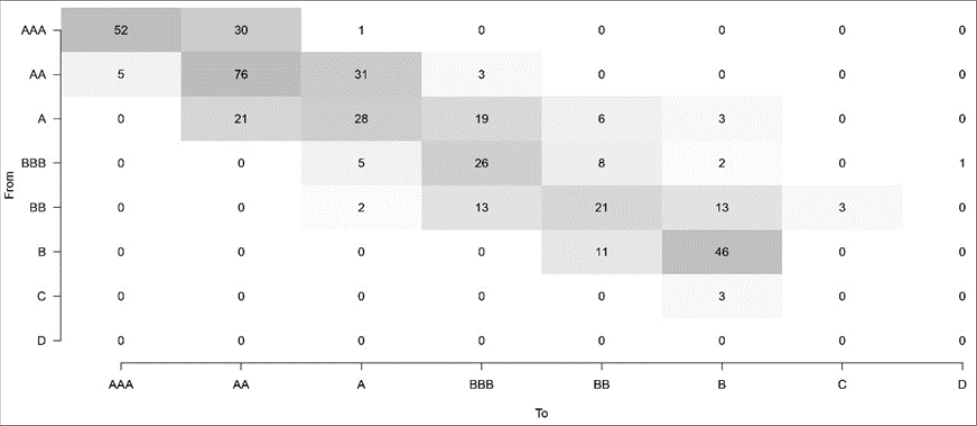 Figure 1
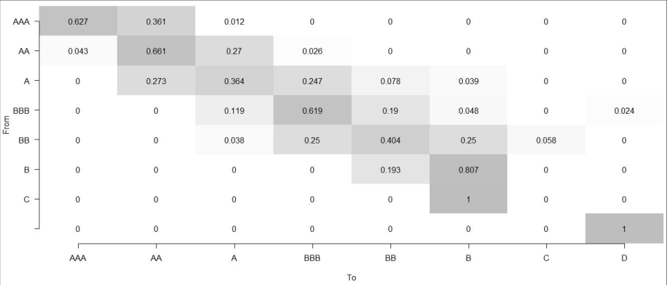 Figure 2
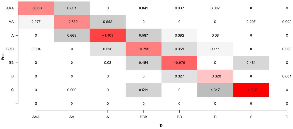 Figure 3
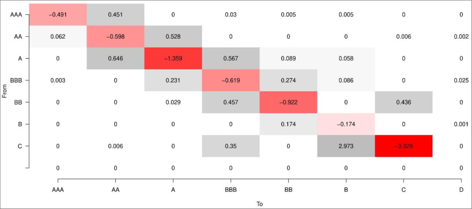 Figure 4
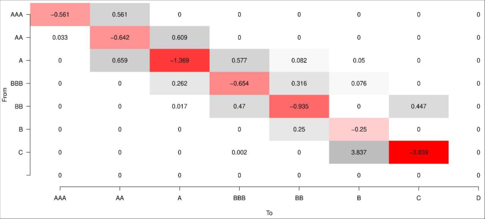 Figure 5
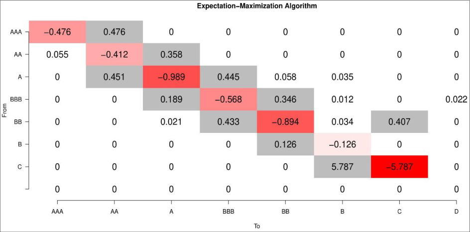 Figure 6
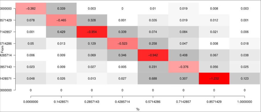 Figure 7
Introduction 1.1 The Maximum Likelihood Estimator
Given any observations set, the maximum likelihood estimator is one of the methods for estimating statistical model parameters. It does this by getting the values of the parameter which maximize the likelihood function. The estimates are referred to as Maximum Likehoood function (MLE). The parameter 𝑄 = [𝑞 𝑖𝑗 ] 𝑖,𝑗 ∈ 𝑆 is the generator matrix. The likelihood function of Q is given by; Taking the logarithm of equation 1 above and then its partial derivative with respect to 𝑞 𝑖𝑗 and equating it to 0 gives the MLE of 𝑄 as; 𝑞 ̂𝑖𝑗 = 𝑁 𝑖𝑗 (𝑇) 𝑅 𝑖 (𝑡) (2) The MLE of parameter 𝑃 ̂ is given as 𝑃 ̂= ( 𝑝̂𝑖 𝑗 ) 𝑖𝑗∈𝑆 Such that;
Where
Where
𝑙 𝑗=1
If the P ̂ shown by equation 3 is embeddable, then the MLE Q ̂ of the generator matrix exists and is obtained by Q ̂= logP ̂. If P ̂ is not embeddable, then there is either existence of Q and other methods of obtaining Q ̂ using the transition estimator P ̂ or else there is no existence of MLE Q ̂.
Materials and Methods
Materials and Methods
The Diagonal and Weighted adjustment
Assuming 𝑙 × 𝑙 transition matrix estimator 𝑃 ̂ given by equation (3) above is not embeddable. The next step is to obtain a matrix 𝑄 ̂ such that 𝑃 ̂= exp (𝑄 ̂). The first thing to do is to be sure that the log function exists for 𝑄 ̂ using the theorem below.
Theorem
Let 𝑃 be 𝑙 × 𝑙 TM and let 𝐹 = 𝑚𝑎𝑥 { (𝑎 -1) 2 + 𝑏 2 , 𝑎 + 𝑏} is an Eigen value of 𝑃, 𝑎, 𝑏 ∈ 𝑅 . Assuming that 𝐹 < 1, then series;
will converge geometrically giving matrix 𝑄 ̂ having row sums equal to 0 and exp(𝑄 ̂) = 𝑃 ̂. The condition 𝐹 < 1 will not be needed if the series absolutely converges. Due to embedding problem, it is not definite that the condition of generator 𝑚𝑎𝑡𝑟𝑖𝑥 𝑄 ̂ to have positive off-diagonal entries though it satisfies exp(𝑄 ̂) = 𝑃 ̂.
The Diagonal Adjustment
Let generator matrix 𝑄 𝐷𝐴 elements given as 𝑞 𝑖𝑗 𝑊𝐴 which will be obtained using the Diagonal Adjustment (DA). The negative value of 𝑄 ̂ will be replaced by 0 since they are usually very small and then the difference added to the diagonal entries so as to preserve the property of row sums totalling to 0. The DA method is given by;
The Weighted Adjustment
Let the generator matrix 𝑄 𝑊𝐴 elements be given as 𝑞 𝑖𝑗 𝑊𝐴 which will be obtained using the Weighted Adjustment method. Let; Letting 𝑒 𝑗 , 𝑒 𝑗 𝐼 to denote the unit vector with 𝑗 𝑡ℎ coordinate equalling to 1 and getting its transpose, it is given that,
The M-Step It is seen that 𝑄 ̃= [𝑞 ̃𝑖𝑗 ] 𝑖,𝑗∈𝑆 where,
Maximizes 𝔼 𝑄 0 [log 𝐿 (𝐶) (𝑄, 𝑌)|𝑋, 𝑄 0 ] hence the new MLE is 𝑄 ̃. Putting 𝑄 ̃= 𝑄 ̃0 and repeating this till there is convergence of sequence. The series of generator matrices {𝑄 𝑘 } 𝑘=1 𝐾 , obtained will depend on the initial matrix generator 𝑄 0 choice hence it is prudent to select it in a way that the det (𝑒 𝑄 𝑘 ) is greater than 0.
The Gibbs sampler (Markov Chain Monte Carlo Method)
This section will demonstrate how to make use of Monte Carlo Chain estimation methods. There are various Monte Carlo Markov Chain methods and the Gibbs Sampler is one of them which will be employed here. The Gibbs Sampler method avoids the non-existence problem of MLE and also makes it very easy to compute. The Gibbs sampler is a method that makes use of samples from joint distribution of some conditional distribution. To understand how this algorithm works its steps are outlined as; Suppose K samples are obtained of 𝑋 = (𝑥 1 , … , 𝑥 𝑛 ) from the joint distribution 𝑝(𝑥 1 , … , 𝑥 𝑛 ). Let the ith sample be given as 𝑋 𝑖 = (𝑥 1 (0) , … , 𝑥 𝑛 (0) ), then the algorithm is:
1. Initialize 𝑋 0 = (𝑥 1 (0) , … , 𝑥 𝑛 (0) ) for 𝑡 = 0.
2. For 𝑖 = 0, … , 𝑘 sample 𝑥 (𝑖+1) by sampling each component of 𝑥 𝑗 (𝑖+1) , 𝑗 = 1, … , 𝑛 and evaluating it using the probability distribution, 𝑝(𝑥 𝑗 (𝑖+1) |𝑥 1 (𝑖+1) , … , 𝑥 𝑗-1 (𝑖+1) , 𝑥 𝑗+1 (𝑖+1) , … , 𝑥 𝑛 (𝑖)
Bayes Theorem
ignoring the constant p(Y) and utilizing (Israel et al., 2001);
Where 𝛼 denotes the proportion, 𝑝(𝜙) the prior distribution and 𝑝(𝜙|𝑌) the posterior distribution which is the conditional distribution of parameter 𝜙 when given data Y. Consider taking a complete data as having discreet time observations 𝑋 = {𝑌(𝑡 1 ), … , 𝑌(𝑡 𝑛 )} observed at time (𝑡 1 = 0, … , 𝑡 𝑛 = 𝑇. An application of 𝑄 and 𝐽 Gibbs sample will be done by drawing 𝐽 from (𝑄, 𝑋) and Q from (𝐽, 𝑋) hence {𝑄 (𝑘) , 𝐽 (𝑘) } 𝑘=1 𝑘 will be obtained where 𝑄 𝑠 denote the generator matrices and 𝐽 𝑠 denote the simulated Markov Chain samples. Given the prior distribution of 𝑄, the gamma distribution proposed is;
Where 𝛼 𝑖𝑗 > 0, 𝑖, 𝑗 ∈ 𝑆 and 𝛽 𝑖 > 0, 𝑖 ∈ 𝑆. Using the likelihood function, given the complete data in equation 1, the posterior of 𝑄 is given as; The Gibbs sampler algorithm is summarized as below Using using data from figure 1 above and running equation 23 using R yields the generator matrix using Gibbs Sampler method is given below;
Hence from norm results 26 above, the norm of Gibbs Sampler method given by 8.207688 is the least hence the most suitable for computing the generator for embeddable 8 × 8 Credit transition Matrix and this paper proposes the Gibbs sampler method as the most accurate for generator matrix approximation for a Credit Transition Matrix.
Figures and tables from the paper
References
5 in the original paper- Carette P. Characterizations of embeddable 3 3 stochastic matrices with a negative eigenvalue. New York J Math. 1995; 1(120):129.
- Hanks E. Ctmcmove: Modeling animal movement with continuous-time discrete-spacemarkov chains. R package version, 2016, 1(3).
- Israel RB, Rosenthal JS, Wei JZ. Finding generators for markov chains via empirical transition matrices, with applications to credit ratings. Mathematical finance. 2001; 11(2):245-265.
- Kingman JFC. The imbedding problem for finite markov chains. Zeitschrift fur Wahrscheinlichkeitstheorie und verwandte Gebiete. 1962; 1(1):14-24.
- Pfeuffer M, Reis GD et al. Capturing model risk and rating momentum in the estimation of probabilities of default and credit rating migrations. arXiv preprint ar. 2018; Xiv:1809.09889.
Cited by 1
From OpenAlex, OpenCitations and reference lists read by Scinovex
- Sovereign Default Forecasting in the Era of the COVID-19 Crisis ↗
Tamás Kristóf · Journal of risk and financial management · 2021
The COVID-19 crisis has revealed the economic vulnerability of various countries and, thus, has instigated the systematic exploration and forecasting of sovereign default risks. Multivariate statistical and stochastic process-based sovereign default risk forecasting has a 50-year developmental history. This article describes a continuous, non-homogeneous Markov chain method as the basis for a COVID-19-related sovereign default risk forecast model. It demonstrates…
❝ 7PDF