A study on generalized invexity in separable Hilbert space

In this paper, it will be shown that two of the main results of Fan seem invalid, and the remaining ones can be proved under any separable Hilbert space, rather than Rn. In addition, some further results are established, which provide some other characterizations for generalized invexity and generalized monotonicity under separable Hilbert spaces.

Illustrations explain the paper; they do not show study data.

AI-generated illustration

↗ Enlarge

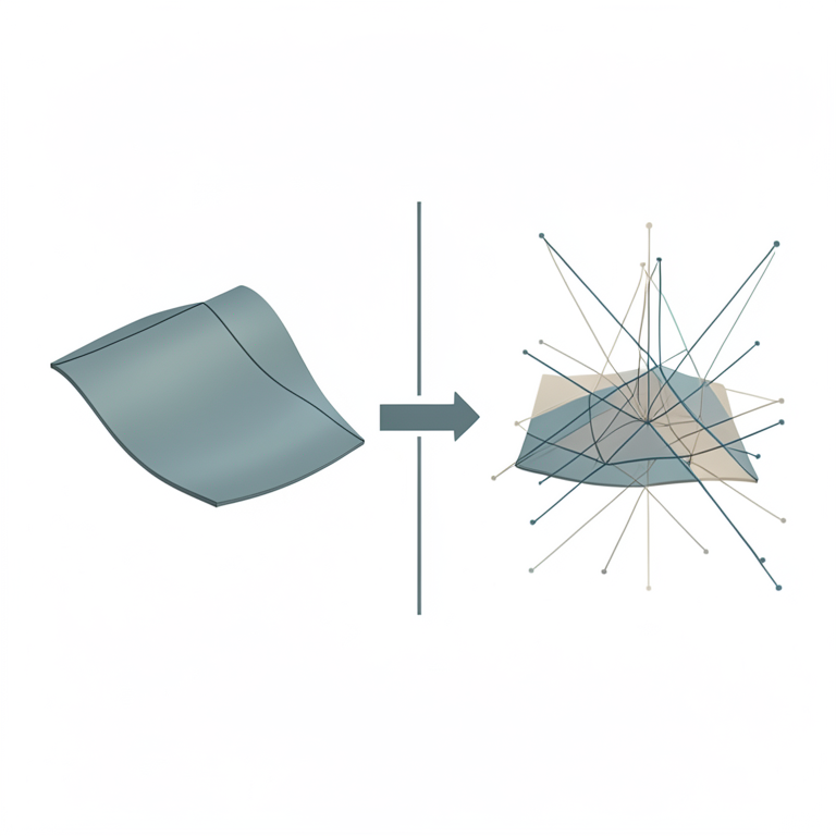
Relationship between Function Invexity and Sub-differential MonotonicityClose ×

AI-generated conceptual illustration (A mathematical representation of a curved surface in a three-dimensional coordinate system). It explains the idea and does not show study data.

Open full-size image ↗

Introduction

An important generalization of convexity is invexity, first introduced by Hanson. In some recently published papers, Soleimani-damaneh has provided some results in invexity analysis. Also in another paper, he has studied the relations between quasi-convexity and pseudoconvexity of a nonsmooth function by means of limiting subdifferentials in Rn. Jabarootian and Zafarani researched the relations between generalized invexity of a non differentiable function and generalized monotonicity of its Clarke generalized sub differential mapping. Fan generalized some results of, using the properties of limiting sub differentials in Rn.

Preliminaries

Let H be a real Hilbert space and let D be a nonempty subset of H. Suppose that 𝑥 is a point not lying in D. Suppose furtherthat there exists a point s in D whose distance to x is minimal. Then s is called the projection of 𝑥 onto D. The set of all such projections is named as the metric projection of x onto D and is denoted byMD (x). Hence MD(𝑥)={s∈D : || 𝑥s || ≤ || 𝑥y || for all y ∈ D } The vector 𝑥 -s determines what we will call a proximal normal direction to D at s. Any nonnegative multiple ζ = λ(x -s), λ ≥ 0, of the proximal normal direction is called a proximal normal to D at s. Hence the proximal normal cone to D at s ∈ D is given by 𝑁 𝐷 𝑃 (s) = {ζ ∈H :∃(λ≥ 0, 𝑥∈ H \ D) such that s ∈ MD(𝑥) &ζ = λ(x -s)}. Suppose that s ∈ D such that s ∉ MD(𝑥) for all 𝑥∉D (for instance, suppose that s ∈ intD), then we define 𝑁 𝐷 𝑃 (s) = {0}.When s ∉D then 𝑁 𝐷 𝑃 (s) remains undefined. A vector ζ ∈ H is said to be a proximal subgradient of h : S ⊆ H → R at 𝑥∈ S if (ζ, -1) ∈𝑁 𝑒𝑝𝑖 ℎ 𝑃 (𝑥, h(𝑥)), Where, epih = {(𝑥, z) : z ≥ h(𝑥)} ⊆ S × R. The set of all proximal subgradient vectors of h at𝑥 is denoted by ∂Ph(𝑥) and is referred to as the proximal sub differential. The function h : R→ R defined by h(𝑥) = -|𝑥| is a simple example of a continuous function having ∂Ph(0) = ∅. Hence, there may exist some points 𝑥, in domain of h such that ∂Ph(𝑥) = ∅. Hence, we define the notion of limiting subdifferentials as follows. In the following definition "wlim" stands for "lim" in the weak topology.

Definition 2.1

A vector d ∈ H is a limiting sub-differential vector of ƒ : S ⊆ H→R at 𝑥∈ S if there exist two sequences {ζi} ⊆ H and { 𝑥i} ⊆ S such that ζi∈∂Pƒ(𝑥i), d = w lim ζi, 𝑥i → 𝑥, and ƒ(𝑥i) →ƒ(𝑥).

The set of all limiting subdifferential vectors of ƒ at x is denoted by ∂Lƒ(𝑥), i.e., ∂Lƒ(𝑥) = {wlim ζi : ζi ∈ ∂Pƒ(𝑥i), 𝑥I →𝑥, ƒ(𝑥i) → f(𝑥)}. The following results concern the closedness and boundedness property of ∂L. A further condition on H(being separable) is required. We recall that a normed vector space is separable if it has a dense countable subset. It is known that a Hilbert space is separable if and only if it has a countable orthogonal basis. Hence it is valid when H = R n . A generalization of the mean value theorem in classic analysis in the presence of limiting subdifferentials. The proofs of the next three theorems can be found.

Theorem 2.1

Let H be separable, and functionƒ: S ⊆ H → R be Lipschitz near 𝑥∈ S. Then ∂Lƒ(𝑥) is nonempty and weaklyclosed. In fact, if 𝑥i →𝑥, di∈∂Lƒ(𝑥i), and di 𝑤 → d, then d ∈∂Lƒ(𝑥).

Theorem 2.2

If ƒ is Lipschitz near 𝑥 with the Lipschitzian constant K, then the set of all limiting subdifferential vectors of ƒ at 𝑥 is bounded by K.

Theorem 2.3

Let function ƒ be locally Lipschitz on a neighborhood of line segment [𝑥, y]. Then for every ∈ > 0 there exists a point z in the ∈neighborhood of [𝑥, y] and ζ ∈ ∂Pƒ(z) such that ƒ(y) -ƒ(𝑥) ≤ 〈ζ, y -𝑥〉 + 𝜖. We follow by introducing the notions of nonsmooth (pre) invex functions, monotone set-valued mappings, and their generalizations in Hilbert spaces. Recall that S ⊆ H is said to be an invex set with respect to mapping η : S × S → H, if u + λη(𝑥, u) ∈ S for each 𝑥, u ∈ S and each λ∈ [0, 1]. Note. Hereafter, unless otherwise specified, we assume that S ⊆ H is a nonempty open invex set with respect to mapping η : S ×S → H. Also ƒ : S → R is a locally Lipschitz (Lipschitz continuous) function on S ⊆ H, where H is a real separable Hilbert space. Definition 2.2 ƒ is said to be (i) preinvex with respect to η on S if for any 𝑥, u ∈ S and any λ ∈ [0, 1], ƒ(u + λη(𝑥, u)) ≤ λƒ(𝑥) + (1 -λ)ƒ(u); (ii) quasi-preinvex with respect to η on S if for any 𝑥, u ∈ S and any λ ∈ [0, 1], ƒ(𝑥) ≤ ƒ(u) ⇒ ƒ(u + λη(𝑥, u)) ≤ ƒ(u); (iii) strictly-quasi-preinvex with respect to η on S if for any 𝑥, u ∈ S and any λ ∈ (0, 1), ƒ(𝑥) < ƒ(u) ⇒ ƒ(u + λη(𝑥, u)) < ƒ(u).

Definition 2.3

ƒ is said to be (i) invex with respect to η on S if for any 𝑥, u ∈ S and any d ∈ ∂Lƒ(𝑥), ƒ(u) -ƒ(𝑥) ≥ 〈d, η(u, 𝑥)〉; (ii) weakly-invex with respect to η on S if for any 𝑥, u ∈ S, there exists d ∈ ∂Lƒ(𝑥) such that ƒ(u) -ƒ(𝑥) ≥ 〈d, η(u, 𝑥)〉; (iii) quasi-invex with respect to η on S if for any 𝑥, u ∈ S, ƒ(u) ≤ ƒ(𝑥) ⇒〈d, η(u, 𝑥)〉≤ 0, ∀d ∈∂Lƒ(𝑥); (iv) weakly-quasi-invex with respect to η on S if for any 𝑥, u ∈ S, ƒ(u) ≤ ƒ(𝑥) ⇒〈d, η(u, 𝑥)〉≤ 0, ∃d ∈ ∂Lƒ(𝑥); (v) pseudo-invex with respect to η on S if for any 𝑥, u ∈ S, 〈𝑑, 𝜂(𝑢, 𝑥)〉 ≥ 0, ∃d ∈ ∂Lƒ(𝑥) ⇒ ƒ(u) ≥ ƒ(𝑥); (vi) strictly-pseudo-invex with respect to η on S if for any 𝑥, u ∈ S with 𝑥 ≠ u, 〈𝑑, 𝜂(𝑢, 𝑥)〉 ≥ 0, ∃d ∈ ∂Lƒ(𝑥) ⇒ ƒ(u) > ƒ(𝑥).

Definition 2.4

A set-valued mapping F : S → 2 H is said to be (i) monotone with respect to η on S if for any 𝑥, u ∈ S and any d ∈ F(𝑥), d1∈ F(u), 〈d 1, 𝜂(𝑥, 𝑢)〉 + 〈𝑑, 𝜂(𝑢, 𝑥)〉 ≤ 0; (ii) quasi-monotone with respect to η on S if for any 𝑥, u ∈ S and any d ∈ F(𝑥), d1∈ F(u), 〈d 1, η(x, u)〉> 0 ⇒〈𝑑, 𝜂(𝑢, 𝑥)〉 ≤ 0; (iii) pseudo-monotone with respect to η on S if for any 𝑥, u ∈ S and any d ∈ F(𝑥), d1∈ F(u),〈d1, η(x, u)〉≥ 0 ⇒〈𝑑, 𝜂(𝑢, 𝑥)〉≤ 0; (iv) strictly-pseudo-monotone with respect to η on S if for any 𝑥, u ∈ S with 𝑥 ≠ u and any d ∈ F(𝑥), d1∈ F(u), 〈d 1, η(x, u)〉 ≥ 0 ⇒〈𝑑, 𝜂(𝑢, 𝑥)〉< 0.

In some of the results of the paper, we need to consider some further assumptions on η. These assumptions are known in invexity literature : (A)for any 𝑥, u ∈ S and any λ

Counter Examples Theorem 2.2.1.

Suppose that η satisfies. If ƒ is quasi-invex with respect to η on S, then it is strictly-quasi-preinvex with respect to the same η on S.

There is no relation between these two theorems. The following counter example shows that the above theorem, is not valid.

Example 2.2.1

Consider S = (-1, 1) ⊆ R. It is clear that S is open and invex with respect to η : S × S → R, defined by η(𝑥, u) = 𝑥 -u. Also, η satisfies. Now consider function ƒ : S → R, defined by 𝑓(𝑥) = { 0, if 𝑥 ∈ (-1, 0] -𝑥2, if 𝑥 ∈ (0, 1). It is not difficult to show that ƒ is Lipschitz on S with a Lipschitzian constant equal to 2. Now we show that ƒ is quasi-invex with respect to η on S. To this end, consider two arbitrary 𝑥, u ∈ S = (-1, 1) such that ƒ(u) ≤ ƒ(𝑥). Therefore, regarding the definition of ƒ, there are two possible cases: case 1. 𝑥∈ (-1, 0], case 2. x, u ∈ (0, 1). In case 1, we have ∂Lƒ(𝑥) = {0} and hence 〈𝑑, 𝜂(𝑢, 𝑥)〉 ≤ 0, for each d ∈ ∂Lƒ(𝑥). Note that the above-defined ƒ is differentiable and hence ∂Lƒ(y) = {ƒˈ(y)} for each y ∈ S. In case 2, we have ∂Lƒ

So far, we have shown that ƒ is quasi-invex with respect to η on S. But in what follows we show that ƒ is not strictly-quasipreinvex with respect to the same η on S. To show this, consider 𝑥= , and λ =

Thus, the above-defined ƒ : S = (-1, 1) → R is quasi-invex with respect to the above-defined η on S, while it is not strictly-quasipreinvex with respect to the same η on S. Implies that there exists δ ∈ (0, 1) such that ƒ(𝑥 𝜆 + μη(𝑥, 𝑥 𝜆 )) ≥ ƒ(y), for each μ ∈ [0, δ], while this conclusion cannot be drawn. In fact, it is valid only when.

𝑙𝑖𝑚 𝜇⟶0 𝑓(𝑥 𝜆 + 𝜇 𝜂 (𝑥, 𝑥 𝜆 ) > 𝑓(𝑦) Theorem 2.2.2

If ∂Lƒ is quasi-monotone with respect to η on S, and ƒ and η satisfy and (C), then ƒ is strictly-quasi-preinvex with respect to the same η on S.

Example 2.2.2

Consider S = (-1, 1) ⊆ R. It is clear that S is open and invex with respect to η : S × S → R, defined by η(𝑥, u) = 𝑥 -u. Now consider function ƒ : S → R, defined by

It is not difficult to show that ƒ is Lipschitz on S with a Lipschitzian constant equal to 2, and ƒ and η satisfy assumptions (A) and (C). It was shown that ƒ is quasi-invex with respect to η on S. Hence, by part (i) of ∂Lƒ is quasi-monotone with respect to η on S. But ƒ is not strictly-quasi-preinvex with respect to the same η on S. Fan assumed, by contradiction, that there exist 𝑥, y ∈ S and λ ∈ (0, 1) such that ƒ(y) < ƒ(𝑥) and ƒ(y + λη(𝑥, y)) ≥ ƒ(𝑥). This assumption is not valid (or sufficient) regarding the definition of strictly-quasi-preinvexity. Indeed, Fan should have assumed that there exist 𝑥, y ∈ S and λ ∈ (0, 1) such that ƒ(y) < ƒ(𝑥) and ƒ(𝑥 + λη(y, 𝑥)) ≥ ƒ(𝑥). However, even this assumption cannot lead to the desired implication.

Extension

In this section, it is shown that the results established can be generalized under any real separable Hilbert space, rather than R n .

Comparing part (ii) in the present paper (or surveying the proof shows that the assumption "η satisfies" of redundant.

Theorem 2.3.1

Suppose that η satisfies. If ƒ is invex with respect to η on S, then ƒ is preinvex with respect to η on S. (ii) If ƒ is preinvex with respect to η on S, then ƒ is weakly-invex with respect to η on S.

Proof

(i) Considering 𝑥, u ∈ S and λ ∈ (0, 1), the invexity hypothesis on S and ƒ, we have ƒ(u) -ƒ(𝑥 + λη(u, 𝑥)) ≥ 〈𝑑, 𝜂(𝑢, 𝑥 + 𝜆𝜂(𝑢, 𝑥))〉 = (1 -λ)〈𝑑, 𝜂(𝑢, 𝑥)〉, ƒ(𝑥) -ƒ(𝑥 + λη(u, 𝑥)) ≥ 〈𝑑, 𝜂(𝑥, 𝑥 + 𝜆𝜂(𝑢, 𝑥))〉 = -λ〈𝑑, 𝜂(𝑢, 𝑥)〉, for any d ∈ ∂Lƒ(𝑥 + λη(u, 𝑥)). Multiplying two above relations by λ and 1 -λ, respectively, and adding the resulted inequalities imply ƒ(𝑥 + λη(u, 𝑥)) ≤ λƒ(u) + (1 -λ)ƒ(𝑥), which completes the proof.

(ii) Suppose that 𝑥, u ∈ S. If η(u, 𝑥) = 0, then the implication is derived easily. Thus suppose that η(u, 𝑥) ≠ 0. Since ƒ is locally Lipschitz, there exists a θ > 0 such that ƒ is Lipschitz on a neighborhood of [𝑥 + λη(u, 𝑥), 𝑥] for each λ ∈ (0, 𝜃 ̅ ), where 𝜃 ̅ = min {1, 𝜃 2𝜂(𝑢,𝑥) }.

Therefore, for each  > 0 there exists a 𝑧 ∈,𝛿 in the  -neighbourhood of line segment [𝑥 + λη(u, 𝑥), 𝑥] and a ζ  ,λ ∈ ∂Pƒ(z  ,λ).

, for each λ ∈ (0, 𝜃 ̅ ). Now if  ↓ 0, then the sequence {𝑧 ∈,𝛿 } has a subsequence, say {𝑧̅ 𝜖,𝛿 }.

This subsequence is bounded and hence it has a weak convergent subsequence, say {𝜁 ̿ , λ}, where 𝜁 ̿ ,λ 𝑤 → 𝑑 ̂λ. We get 𝑑 ̂λ∈ ∂Lƒ(𝑥 ̂λ). Therefore, by  ↓ 0, we have, ƒ(u) -ƒ(𝑥) ≥ 〈𝑑𝜆, 𝜂(𝑢, 𝑥)〉. Now if λ ↓ 0, then 𝑥 ̂λ→ 𝑥 and regarding the above discussions without loss of generality we can assume that 𝑑 ̂λ 𝑤 →d, where d ∈ ∂Lƒ(𝑥). Therefore ƒ(u) -ƒ(𝑥) ≥ 〈𝑑, 𝜂(𝑢, 𝑥)〉, for some d ∈ ∂Lƒ(𝑥), and the proof is complete.

Theorem 2.3.2

If ƒ is quasi-preinvex with respect to η on S, then ƒ is weakly-quasi-invex with respect to η on S.

Proof

Suppose that u, 𝑥∈ S and ƒ(u) ≤ ƒ(𝑥). If η(u, 𝑥) = 0, then the implication is derived simply. Thus suppose that η(u, 𝑥) ≠ 0. By quasi-preinvexity, we have ƒ(𝑥) -ƒ(𝑥 + λη(u, 𝑥)) ≥ 0,for each λ ∈ (0, 1). Since ƒ is locally Lipschitz, there exists a θ > 0 such that ƒ is Lipschitz on a neighborhood of [𝑥 + λη(u, 𝑥), 𝑥] for each λ ∈ (0, 𝜃 ̅ ), where 𝜃 ̅ = min{1, subsequence is bounded with regard to 〈𝑑 λ, 𝜂(𝑢, 𝑥)〉 ≤ 0. Now if λ ↓ 0, then 𝑥 ̂λ → x and regarding the above discussions without loss of generality we can assume that 𝑑 ̂λ 𝑤 → d, where d ∈ ∂Lƒ(𝑥). Therefore 〈𝑑, 𝜂(𝑢, 𝑥)〉 ≤ 0,for some d ∈ ∂Lƒ(𝑥), and the proof is complete. The following theorem corrects and generalizes. The assumption of the following theorem shows that replacing the assumption "being locally Lipschitz" with "being Lipschitz" is more exact.

Theorem 2.3.3

Suppose that ƒ is Lipschitz and η satisfies assumption (A). If ƒ is quasi-invex with respect to η on S, then ƒ is quasi-preinvex with respect to η on S.

Proof.

By contradiction suppose that ƒ is not quasi-preinvex, and there exist 𝑥, u ∈ S and a λ ∈ (0, 1) such that ƒ(𝑥) ≤ ƒ(u) and ƒ(u + λη(𝑥, u)) > ƒ(u). Setting 𝑥̅ = u + λη(𝑥, u), we get ƒ(𝑥̅ ) > ƒ(u). Since ƒ is Lipschitz, it is continuous on S and hence there exists a δ1∈ (0, 1) such that ƒ(u + θ (𝑥̅ -u)) > ƒ(u), for each θ ∈ [δ1, 1], and ƒ(𝑥̅ ) > ƒ(u + δ1(𝑥̅ -u)). Hence, setting δ = λδ1, we have δ ∈ (0, λ), ƒ(u + μ η(𝑥, u)) > ƒ(u), for each μ ∈ [δ, λ], and ƒ(𝑥̅ ) > ƒ(u + δη(𝑥, u)).

Since ƒ is Lipschitz on a neighborhood of [u + δη(𝑥, u), 𝑥̅ ], for each  > 0 there exists a z in the  -neighborhood of line segment [u + δη(𝑥, u), 𝑥̅ ] and a ζ∈ ∂Pƒ(𝑧 ∈ ) such that ƒ(𝑥̅ ) -ƒ(u + δη(𝑥, u)) ≤ 〈𝜁𝜖, 𝑥̅ -(𝑢 + 𝛿 𝜂(𝑥, 𝑢))〉 +  = (λ -δ)〈𝜁𝜖, 𝜂(𝑥, 𝑢)〉 +  . Now if  ↓ 0, then the sequence {z} has a subsequence, say {𝑧̅ }, such that 𝑧̅ → 𝑥 ̂ where 𝑥 ̂ belongs to the line segment [u + δη(x, u), 𝑥̅ ]. Let the subsequence of {ζ} which is corresponding to {𝑧̅ } be denoted by {𝜁 ̅ }. This subsequence is bounded and hence it has a weak convergent subsequence, say {𝜁 ̿ }, where 𝜁 ̿ 𝑤 → 𝑑 ̂. We get 𝑑 ̂∈ ∂Lƒ(𝑥 ̂). Therefore, by  ↓ 0, we have 0 <ƒ(𝑥̅ ) -ƒ(u + δη(𝑥, u)) ≤ (λ -δ)〈𝑑 ̂, 𝜂(𝑥, 𝑢)〉. Hence 〈𝑑 ̂, 𝜂(𝑥, 𝑢)〉> 0. On the other hand, since 𝑥 ̂∈ [u + δη(x, u),𝑥̅ ], there exists α ∈ [0, 1] such that 𝑥 ̂ = αu + αδη(𝑥, u) + (1 -α)𝑥̅ = αu + αδη(𝑥, u) + (1-α)u + (1-α) λη(𝑥, u) = 𝑢 + (αδ + λ -αλ)η(𝑥, u). Thus defining 𝜆 ̅ = αδ + λ -αλ, we have 𝜆 ̅ ∈ [δ, λ] and 𝑥 ̂ = u + 𝜆 ̅ η(𝑥̅ , Therefore, we have ƒ(𝑥 ̂) > ƒ(u) ≥ ƒ(𝑥). Thus by the assumption of the theorem we get 〈𝑑, 𝜂(𝑥, 𝑥 ̂)〉 ≤ 0, ∀d ∈ ∂Lƒ(𝑥 ̂). On the other hand, by assumption (A) and the above inequality, for each d ∈ ∂Lƒ(𝑥 ̂) we have 0 ≥ 〈𝑑, 𝜂(𝑥, 𝑥 ̂)〉 = 〈𝑑, 𝜂(𝑥, 𝑢 + 𝜆𝜂(𝑥̅ , 𝑢))〉 = (1 -λ) -d, η(𝑥, u), which implies that 〈𝑑, 𝜂(𝑥, 𝑢)〉 ≤ 0, ∀d ∈ ∂Lƒ(𝑥 ̂). This contradicts. Hence, we have ƒ(u + λη(𝑥, u)) ≤ ƒ(u), for each [0, 1). The above inequality for λ = 1 is derived regarding the continuity of ƒ, and the proof is completed.

Theorem 2.3.4

Suppose that η satisfies. If ƒ is pseudo-invex with respect to η on S, then ƒ is strictly-quasi-preinvex with respect to η on S.

Proof

By contradiction suppose that ƒ is not strictly-quasi-preinvex, then there exist 𝑥, u ∈ S and a λ ∈ (0, 1) such that ƒ(𝑥) < ƒ(u) and ƒ(u + λη(𝑥, u)) ≥ ƒ(u). Regarding the pseudo-invexity of ƒ, we have η(u, 𝑥) ≠ 0. Setting 𝑥̅ = u + λη(𝑥, u), we get ƒ(𝑥̅ ) ≥ ƒ(u) > ƒ(𝑥). By the pseudoinvexity assumption we have 〈𝑑, 𝜂(𝑥, 𝑥̅ )〉 < 0 for each d ∈ ∂Lƒ(𝑥̅ ). By assumption (A), we have 0 >〈𝑑, 𝜂(𝑥, 𝑥̅ )〉 = 〈𝑑, 𝜂(𝑥, 𝑢 + 𝜆𝜂(𝑥, 𝑢))〉 = (1 -λ) 〈𝑑, 𝜂(𝑥, 𝑢)〉 And 〈𝑑, 𝜂(𝑢, 𝑥̅ )〉 = 〈𝑑, 𝜂(𝑢, 𝑢 + 𝜆𝜂(𝑥, 𝑢))〉 = -λ 〈𝑑, 𝜂(𝑥, 𝑢)〉. Hence 〈𝑑, 𝜂(𝑢, 𝑥̅ )〉> 0 for each d ∈ ∂Lƒ(𝑥̅ ), and thus we have ƒ(𝑥̅ ) ≤ ƒ(u) by pseudo-invexity assumption. Therefore ƒ(𝑥̅ ) = ƒ(u). On the other hand, since S is open and ƒ is locally Lipschitz on S, there exists a 0 <𝛿 ̅ < 1 such that Bδ(𝑥̅ ) ⊂ S and ƒ is Lipschitz on a neighborhood of [𝑥̅ + δη(u, 𝑥̅ ), 𝑥̅ ] ⊆Bδ(𝑥̅ ), for each δ ∈ (0, 𝛿 ̅ ]. Now, for each  > 0 there exists a 𝑧 ∈,𝛿 in the  -neighborhood of the line segment [𝑥̅ + δη(u, 𝑥̅ ), 𝑥̅ ] and a vector d,δ∈ ∂Pf(𝑧 ∈,𝛿 ) such that ƒ(𝑥̅ ) -ƒ(𝑥̅ + δη(u, 𝑥̅ )) ≤ -δ 〈𝑑 ∈,𝛿 , 𝜂(𝑢, 𝑥̅ )〉 +  . Now if  ↓ 0, then the sequence {𝑧 ∈,𝛿 } has a subsequence, say { Thus there exists a vector 𝑥 ̂ and a μ ∈ (0, 1) such that S ∋𝑥 ̂ = 𝑥̅ + μη(u, 𝑥̅ ) and ƒ(𝑥 ̂) > ƒ(𝑥̅ ) = ƒ(u). Hence, using the pseudo-invexity assumption we get 〈𝜋, 𝜂(𝑢, 𝑥 ̂)〉< 0 and 〈𝜋, 𝜂(𝑥̅ , 𝑥 ̂)〉< 0 for each π ∈ ∂Lƒ(𝑥 ̂). Therefore,

This is an obvious contradiction, which completes the proof.

Theorem 2.3.5 (i) If ƒ is invex with respect to η on S, then ∂Lƒ is monotone with respect to η on S. (ii) If ƒ is Lipschitz and then the reverse of (i) holds. Proof (i) Consider arbitrary 𝑥, u ∈ S. By invexity hypothesis, we have ƒ(𝑥) -ƒ(u) ≥ 〈𝑑, 𝜂(𝑥, 𝑢)〉 for each d ∈ ∂Lƒ(u), and ƒ(u) -ƒ(𝑥) ≥〈𝑑 ̅ , 𝜂(𝑢, 𝑥)〉 for each 𝑑 ̅ ∈ ∂Lƒ(𝑥). Thus, we have 〈𝑑, 𝜂(𝑥, 𝑢)〉 + 〈𝑑 ̅ , 𝜂(𝑢, 𝑥)〉 ≤ 0 for each d ∈ ∂Lƒ(𝑥) and 𝑑 ̅ ∈ ∂Lƒ(u), and the proof is complete. (ii) Consider arbitrary 𝑥, u ∈ S and arbitrary d ∈ ∂Lƒ(u). We need to show that ƒ(𝑥) -ƒ(u) ≥ 〈𝑑, 𝜂(𝑥, 𝑢)〉. Since ƒ is Lipschitz on a neighborhood of [u + η(𝑥, u), u + ). Therefore, regarding θ1, θδ> 0, we have 〈𝑑, 𝜂(𝑥, 𝑢)〉 ≤ <d1, η(𝑥, u)> And 〈𝑑, 𝜂(𝑥, 𝑢)〉 ≤,< 𝑑 𝛿 , η(𝑥, u)>, for each δ ∈ (0, ). Which imply that ƒ(𝑥) -ƒ(u + δη(𝑥, u)) ≥ (1 -δ) 〈𝑑, 𝜂(𝑥, 𝑢)〉. Thus, since ƒ is continuous by δ ↓ 0, we get ƒ(𝑥) -ƒ(u) ≥ 〈𝑑, 𝜂(𝑥, 𝑢)〉, and the proof is complete, when η(𝑥, u) ≠ 0. If η(𝑥, u) = 0, by assumption (B), we have ƒ(𝑥) -ƒ(u) ≥ ƒ(u + η(𝑥, u)) -ƒ(u) = 0 = 〈𝑑, 𝜂(𝑥, 𝑢)〉, and the proof is complete. Part (ii) of the following theorem corrects and generalizes part (ii). Theorem 2.3.6 (i) If ƒ is quasi-invex with respect to η on S, then ∂Lƒ is quasi-monotone with respect to η on S. (ii) If ƒ is Lipschitz and ∂Lƒ is quasi-monotone with respect to η on S, then ƒ is quasi-preinvex with respect to η on S.

Proof

The proof of part (i) is straightforward. To prove part (ii), consider 𝑥, u ∈ S such that ƒ(𝑥) ≤ ƒ(u). Since ƒ is continuous, we need to prove that ƒ(u + λη(𝑥, u)) ≤ ƒ(u), for each λ ∈ (0, 1). By contradiction suppose that ƒ(u + 𝜆 ̅ η(𝑥̅ , u)) > ƒ(u) ≥ ƒ(𝑥), for some 𝜆 ̅ ∈ (0, 1). Therefore, regarding assumption (C), we have ƒ(u + 𝜆 ̅ η(𝑥, u)) > ƒ(u + η(𝑥, u)). Since ƒ is continuous, regarding the two last relations, we have ƒ(u + λ1η(𝑥, u)) > ƒ(u), and ƒ(u + λ2 η(𝑥, u)) > ƒ(u + η(𝑥, u)) for some λ1 ∈ (0, 𝜆 ̅ ) and λ2 ∈ (𝜆 , 1). Since ƒ is Lipschitz on a neighborhood of [u, u + λ1 η(𝑥, u)] and hence for each  > 0 there exists a z in the  -neighborhood of the line segment [u, u + λ1η(𝑥, u)] and a vector d∈ ∂Pƒ(z) such that ƒ(u + λ1η(𝑥, u)) -ƒ(u) ≤ λ1 d, η(𝑥, u) +  . Now if  ↓ 0, then the sequence {z} has a subsequence, say {𝑧̅ }, such that 𝑧̅ → c1∈ [u, u + λ1η(𝑥, u)]. Let the subsequence of {d} which is corresponding to {𝑧̅ } be denoted by {𝑑 ̅ }. This subsequence is bounded and hence it has a weak convergent subsequence, say {𝑑 ̿ }, where 𝑑 ̿ 𝑤 →d1. We get d1∈ ∂Lƒ(c1). Therefore, we have c1 = u + θ1η(𝑥, u) for some θ1∈ [0, λ1], and 0 <ƒ(u + λ1η(𝑥, u)) -ƒ(u) ≤ λ1 d1, η(𝑥, u). In a similar way, there exists a c2∈ [u + η(𝑥, u), u + λ2η(𝑥, u)) and an d2∈ ∂Lƒ(c2) such that c2 = u + θ2η(𝑥, u) for some θ2∈ [λ2, 1], and 0 <ƒ(u + λ2η(𝑥, u)) -ƒ(u + η(𝑥, u)) ≤ (λ2 -1) <d2, η(𝑥, u)>. Hence, <d1, η(𝑥, u)> 0 and <d2, η(𝑥, u)> < 0. By assumption (A) and we have <d1,η(c2, c1)> = <d1, η(u+θ2η(𝑥, u), u+θ1η(𝑥, u) = <d1,η(u + θ1η(𝑥, u) + (θ2 -θ1)η(𝑥, u), u + θ1η(𝑥, u))> = <d1, η(u + θ1η(𝑥, u) + Therefore we get <d1, η(c2, c1)> > 0 and <d2, η(c1, c2) > > 0. These contradict quasi-monotonicity of ∂Lƒ, and completes the proof.

Conclusion

This paper provides us the characterization of basic solutions as the extreme point of the set of feasible solutions which shows that if there is a feasible solution for an IP then there must be a basic feasible solution. This property has been strengthened and characterizes the basic optimal solutions of an IP and guarantees that a basic optimal solution can be constructed from an optimal solution and shows how the invexity is done in separable Hilbert space.

1. Hanson MA. On sufficiency of the Kuhn-Tucher conditions, J. Math. Anal. Appl. 1981; 80:545-550.
2. Jabarootian T, Zafarani J. Generalized invariant monotonicity and invexity of non-differentiable functions, J. Global Optim. 2006; 36:537-564.
3. Karamardian S, Schaible S. Seven kinds of monotone maps, J Optim. Theory. Appl. 1990; 66:37-46.
4. Luc DT. Charactrization of quasiconvex functions, Bull. Aust. Math. Soc. 1993; 48.
5. Mordukhovich BS. Variations Analysis and Generalized Differentiation, I: Basic Theory, in: Grundlehren Series (Fundamental Principles of Mathematical Sciences), Springer. 2006; 6.
6. Mordukhovich BS. Variations Analysis and Generalized Differentiation, II: Applications, in: Grundlehren Series (Fundamental Principles of Mathematical Sciences). 2006; 331.
7. Peng JW. Criteria for generalized invexmonotonicities without condition C, European J Oper. Res. 2006; 170:667-671.
8. Ruiz-Garzón G, Osuna-Gómez R, Rufian-Lizana A. Generalized invex monotonicity, European J Oper. Res. 2003; 144:501512.
9. Soleimani-damaneh M. Characterization of non smooth quasi convex and pseudo convex functions, J Math. Anal. Appl. 2007; 330:1387-1392.
10. Soleimani-damaneh M. Multiple-objective programs in Banach spaces: Sufficiency for (proper) optimality, Nonlinear Anal. 2007; 67(3):958-962.
11. Sindhu V. Decomposition of α continuity and α*g continuity and g # closed sets in topology. ISSN: 2320 -0294, International Journal of Engineering Science and Mathematics. 2017; 6(2):38-47.