
Research article · 2019 · Full text
International Journal of Statistics and Applied MathematicsModeling household water demands using sinusoidal models
Volume 4(6) · Pages 128–132
Research areasWater resources management and optimization
Abstract
Author-writtenHousehold water in Kenya is used in agricultural activities, industrial activities and other uses. A lot of water is consumed by indoor appliances. The water management strategy affects the household demand for water. The future demand of water in Kenyan towns has remained uncertain. Therefore this study sought to model household water demand using the non- parametric model in the spectral domain. This study largely relied on the secondary data that was collected from Gusii Water and Sanitation Company (GWASCO) situated in Kisii town. This study inspected the data for trend by applying Mann Kendal trend test and it was realized that the p-value = 0.012< Siginificance level, α = 5% indicating that the water demand data had a trend. The parameters of the sinusoidal model was estimated and they were: B1 = 90.28176, B2 = 69.06094 and μ = 3586.94540 The developed model was used in conducting in sample forecasting. The forecasted values were plotted together with those of GWASCO and comparison was made. This study noted no significant difference in the plots. Therefore, the model was employed in conducting out of sample forecasting. The out sample forecasted values increased with time. This study concluded that the water data had a trend, had periodic variations hence could be modeled using the sinusoids and that the forecasts increased with time.
Summary
Source-checkedPlain-language reading of the full paper, prepared with AI and checked against the text. Each point links to the authors' own words.
Why it matters
- Household water in Kenya is utilized for various purposes, including industrial and agricultural activities, with a significant amount used by indoor appliances. View evidence ↗
- There is uncertainty regarding the future demand for water within Kenyan towns. View evidence ↗
- An upward trend in Kenyan population estimates suggests that the demand for water in the country is continuously increasing. View evidence ↗
The question
- The study aimed to model household water demand using a non-parametric model within the spectral domain. View evidence ↗
What they did
- The research utilized secondary data obtained from the Gusii Water and Sanitation Company (GWASCO) in Kisii town. View evidence ↗
- The study analyzed a sample size of 97 observations, which is an odd number. View evidence ↗
- The Cox-Stuart (C-S) test was employed to detect non-random periodic patterns in the data. View evidence ↗
- An F-test was conducted to identify significant harmonic waves (HWs) to determine the parameters for the sinusoidal model. View evidence ↗
What they found
- The Cox-Stuart test resulted in a p-value of 0.00001141, which is less than the 0.05 significance level, indicating that the household water data has a periodic trend. View evidence ↗
- F-test results showed that only the 33rd harmonic wave was significant, while all others were insignificant. View evidence ↗
- The mean of the collected water demand data was found to be 3586.94540. View evidence ↗
- The estimated parameters for the suitable sinusoidal model were B1 = 90.28176, B2 = 69.06094, and a mean (mu) of 3586.94540. View evidence ↗
- In-sample forecasting showed no significant difference between the forecasted figures and the collected data, suggesting the model is suitable. View evidence ↗
- Out-of-sample forecasts indicated that water demand values increased over time. View evidence ↗
What it means
- The authors concluded that the developed sinusoidal model is suitable for describing the household water demand data. View evidence ↗
- The authors recommend that GWASCO use the developed model to forecast future water demand to better match customer needs. View evidence ↗
- The authors suggest that future research should compare these results with other methods, such as Box-Jenkins modeling or double exponential smoothing. View evidence ↗
- The authors note that future studies could use residual plots or the coefficient of determination to further validate model suitability instead of relying solely on in-sample forecasting. View evidence ↗
Visual summary
2 visualsIllustrations explain the paper; charts are replotted from the paper's own table values.
Sinusoidal Modeling Workflow
AI-generated conceptual illustration (residential water meter and plumbing system). It explains the idea and does not show study data.
View source evidence ↗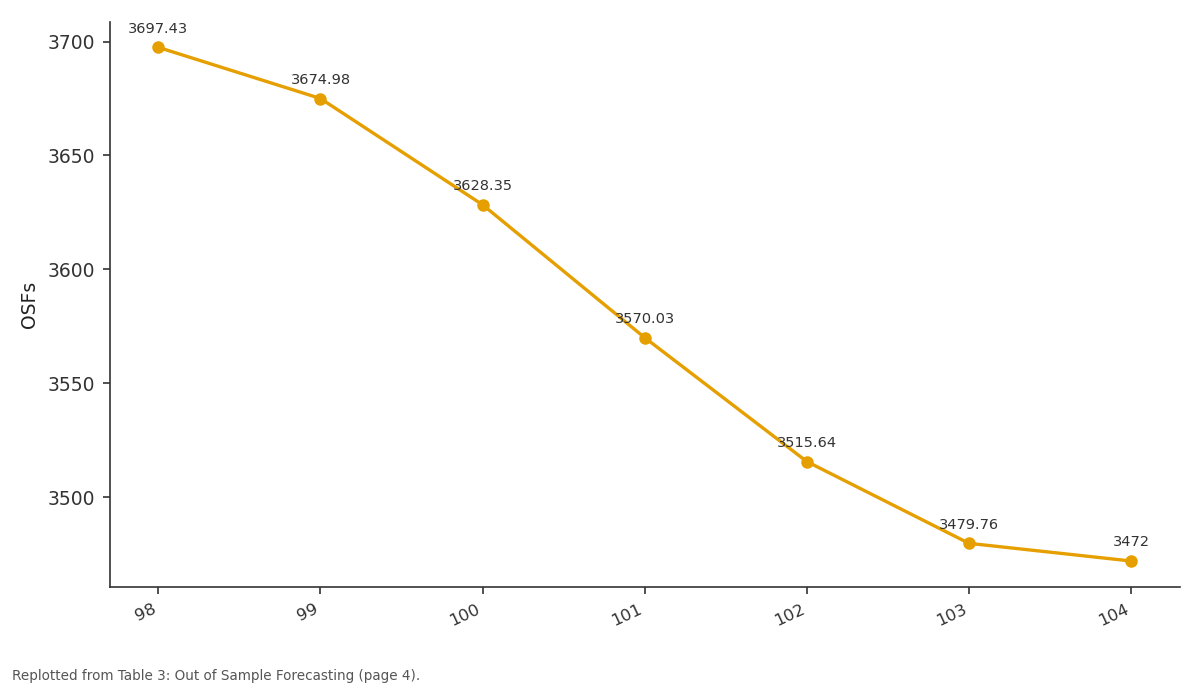
OSFs: 98 vs 99 vs 100 vs 101 vs 102
Replotted from Table 3 (page 4) of the original paper. Every bar is the paper's own table value.
View source evidence ↗Figures & tables
From the original paper Table 1
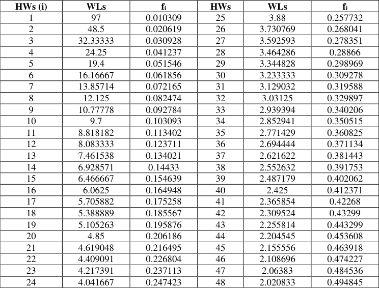 Table 2
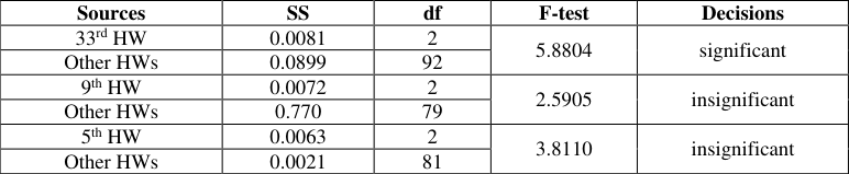 Table 3
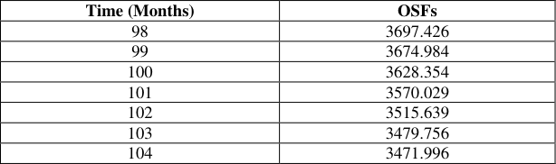 Table 3
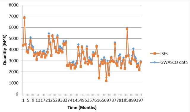 Figure 1
Introduction
Water is considered to be one of the crucial resources in the survival of living things. Human beings rely on water to conduct household chores. The location, function and household personal preferences are the main contributors in the determination of household water demand. The quantity of water demanded per capita has been provided by various organizations. According to Kenya Ministry of Water Resource Management and Development, the country's water supply stands at 647M 3 per capita. World Resource Institute estimates the volume of water demanded to be 590M 3 per capita. This indicates a huge variation in the estimates by various institutions [1,2] . The procedure of unraveling the quantity of water demanded in a country relies heavily on the population estimates. The Kenyan population estimates have been on the upward trend indicating an ever increasing demand of water in the country. This has led to the development of institutions in various parts of the country to help in the management of the household water demand [2] . In statistics, frequency domain refers to the analysis of the mathematical functions/signals with respect to the frequency rather than time [3] . The detail of determining the spectral density of a sample of population data is very old; this was applied by the first astronomers who tried to study the length of the year and the period of the moon. This entailed the determination of the maxima and/or estimation of the period [4] . The first significant frequency estimation problem took place in the 19 th century where the probability theory and the use of Fourier transform came into being. In the frequency estimation process, the model might contain a single cosine with amplitude, phase and a frequency contaminated by the noise error with unknown variance. Basically a researcher is interested in the amplitude, phase or noise variance [4,5] .
Material and Methods
Material and Methods
Cox-Stuart Trend Tests
According to [5] , C-S test is normally employed to detect the non-random pattern, that is the periodic patterns. C-S test compares the first half and the second half of the sample data. When the data has a down ward trend, the observatons in the first half are expected to be greater than the observation in the second half. When the data has upward trend, the observations in the first half are expected to be smaller than the observations in the second half. When the data in question has no trend, then the researcher should expect smaller differences between the two halves of the sample data due to the randomness of the data. To perform the C-S test, the sample differences are computed as shown below;
The hypotheses tested at the significance level (α) are: H 0 : There is no periodic trend in the household water data H A : There is periodic trend in the household water data
Sinusoidal modeling
According to [6] , the periodicities were modeled using the sinusoidal model of the form:
In this equation 𝜇, 𝐴 and 𝑃 cannot be estimated by the standard least square method. To achieve this estimator we expanded as shown below;
Where 𝐵 1 = A * cos(𝑃) and 𝐵 2 = 𝐴 * sin(𝑃) Hence the structure of the sinusoidal model becomes:
Where the parameters 𝜇, 𝐵 1 and 𝐵 2 can be estimated by the method of least squares estimation process.
Therefore the Amplitude (A) can be estimated by
In some cases the amplitudes of the peaks and the troughs are rarely equal, then the sine wave model can be re-written using the Fourier series model: ).
Forecasting
This study used the developed model to forecast the future demand of house water data. The model used was of the following form: From table 4 above, it can be deduced that the p-value = 0.00001141 < the significance level (α) = 0.05. Therefore this study can reject the null hypothesis in favor of the alternative hypothesis and conclude that the household water data has a periodic trend.
Sinusoidal modeling
Since the sample size of this study consisted of 97 observations (odd number) the sinusoidal model structure suitable for this study is indicated below.
The maximum number of the HWs for the observations is Some of the HWs, WLs and frequencies are as indicated in the table below: As it can be noted from table above the highest frequency was 0.49 followed by 0.48 and the least 0.01. The longest WL was 97 followed by 48.50 and the least was 2.02 and the least HW was 1 followed by 2 in that order, the highest was 48. This study further conducted an estimation process of the parameters of the sinusoidal model in (3.13) above using the Fourier series estimation process. Some of the parameters are as indicated below.
𝐵 ̂ 11 = -0.07920 , 𝐵 ̂21 = -0.03755 𝐵 ̂12 = 0.04490 , 𝐵 ̂22 = 0.052008 𝐵 ̂1,33 = 90.28176 , 𝐵 ̂2,33 = 69.06094 𝐵 ̂1,94 = -0.00892 , 𝐵 ̂2,95 = 0.00567 𝜇̂= 3586.94540
The mean of the collected data is 3586.94540 as indicated in the estimated parameters above. This study took a step further and conducted the F-test to determine the significant HWs so that we could determine the parameters of the sinusoidal model. The Ftest is as indicated in the table below: From the F-tests, it was only the 33 rd HW that was significant, others were insignificant, therefore the parameters of the sinusoidal model was chosen to be 𝐵 ̂1,33 = 90.28176, 𝐵 ̂2,33 = 69.06094 and 𝜇̂= 3586.94540 and therefore the suitable sinusoidal model for the GWASCO water supply data would be:
𝑌 ̂𝑡 = 3586.9454 + 69.06094 cos(0.5236𝑡) + 90.2817 sin(0.5236𝑡)
Forecasting
In-sample forecasting was conducted and comparison was made between the forecasted figures and that of the collected data. The plots are indicated in figure 1 below. From the plot in figure 1 above it can be noted that there was no significant difference in the plots indicating the suitability of the model in forecasting. This study took a step further and conducted the OSFs (future forecasts) 9 months for the next using the developed model. The forecasts are as indicated in the table below.
Conclusions
From Cox-Stuart test, this study concluded that the data had a trend and thus could be modeled using the spectral analysis to a data set with a trend. The spectral analysis was conducted and this study realized that the data had periodic variations and thus the researcher concluded that the data could be modeled using the sinusoids.
In the modeling of the data, this study realized that the number of observations were odd in number (97 months) and thus the researchers estimated and concluded that the number of HWs were 48. The parameters of the model were estimated and the F-test was conducted to determine which of the HWs were significant. It was realized that the 33 rd HW was significant and thus determined the structure of the model parameters. Thus the parameters were concluded to be B 1 = 90.28176 and B 2 = 69.06094. The mean of the data was 3586.9454 M 3 . Thus this study concluded that the model took the following form; 𝑌 ̂𝑡 = 3586.9454 + 69.06094 cos(0.5236𝑡) + 90.2817 sin(0.5236𝑡) In sample forecasts was conducted by this study. This study noted no significance difference in the plots of GWASCO water demand data and that of the in-sample forecasts. This study concluded that the fitted model was suitable to be used to describe the data. In effect to the aforementioned, this study used the model to provide 9 months ahead forecast.
Recommendations
From this research, we were able to determine the trend of the data using the Cox-Stuart trend test, but the same results could be realized if ordinary least square method in trend determination is employed. This study employed spectral analysis of sinusoids in modeling the water demand but future researchers could employ other methods like Box-Jenkins modeling approach and double exponential smoothing methods and make comparison to determine if the same implications could be realized. The model developed in this study could also be investigated to determine if it will be suitable in forecasting the water demand data in other regions of the country. Additionally, this study used the in-sample forecasting as a method of determining if the developed model actually represents the true picture of the collected time series data. Future researchers could try other methods like using the residual plots and/ or the coefficient of determination method in determining the suitability of a model. Finally, Gusii Water and Sanitation Company (GWASCO) could use the developed model in conducting the future forecasts.
This will aid in determining the quantity of water demanded by its customers and thus the company will try to match the amount of water demanded. The methods used in this study in modeling the water demand time series data could also be used in other regions by future researchers in modeling the water data.
Acknowledgement
Special thanks to all the individuals who made the research process a success. We are also indebted to Gusii Water and Sanitation Company (GWASCO) because they availed the household water demand data hence contributing immensely to the success of this research.
Figures and tables from the paper
| Description | Value |
|---|---|
| Cox-Stuart Statistic | 4.8655 |
| P-value | 0.00001141 |
| Significance level(α) | 0.05 |
Table text extracted from the original PDF; superscript letters are shown inline. The original table image is below.
View original table image
| HWs (i) | WLs | fi | HWs | WLs | fi |
|---|---|---|---|---|---|
| 1 | 97 | 0.010309 | 25 | 3.88 | 0.257732 |
| 2 | 48.5 | 0.020619 | 26 | 3.730769 | 0.268041 |
| 3 | 32.33333 | 0.030928 | 27 | 3.592593 | 0.278351 |
| 4 | 24.25 | 0.041237 | 28 | 3.464286 | 0.28866 |
| 5 | 19.4 | 0.051546 | 29 | 3.344828 | 0.298969 |
| 6 | 16.16667 | 0.061856 | 30 | 3.233333 | 0.309278 |
| 7 | 13.85714 | 0.072165 | 31 | 3.129032 | 0.319588 |
| 8 | 12.125 | 0.082474 | 32 | 3.03125 | 0.329897 |
| 9 | 10.77778 | 0.092784 | 33 | 2.939394 | 0.340206 |
| 10 | 9.7 | 0.103093 | 34 | 2.852941 | 0.350515 |
| 11 | 8.818182 | 0.113402 | 35 | 2.771429 | 0.360825 |
| 12 | 8.083333 | 0.123711 | 36 | 2.694444 | 0.371134 |
| 13 | 7.461538 | 0.134021 | 37 | 2.621622 | 0.381443 |
| 14 | 6.928571 | 0.14433 | 38 | 2.552632 | 0.391753 |
| 15 | 6.466667 | 0.154639 | 39 | 2.487179 | 0.402062 |
| 16 | 6.0625 | 0.164948 | 40 | 2.425 | 0.412371 |
| 17 | 5.705882 | 0.175258 | 41 | 2.365854 | 0.42268 |
| 18 | 5.388889 | 0.185567 | 42 | 2.309524 | 0.43299 |
| 19 | 5.105263 | 0.195876 | 43 | 2.255814 | 0.443299 |
| 20 | 4.85 | 0.206186 | 44 | 2.204545 | 0.453608 |
| 21 | 4.619048 | 0.216495 | 45 | 2.155556 | 0.463918 |
| 22 | 4.409091 | 0.226804 | 46 | 2.108696 | 0.474227 |
| 23 | 4.217391 | 0.237113 | 47 | 2.06383 | 0.484536 |
| 24 | 4.041667 | 0.247423 | 48 | 2.020833 | 0.494845 |
Table text extracted from the original PDF; superscript letters are shown inline. The original table image is below.
View original table image
| Sources | SS | df | F-test | Decisions |
|---|---|---|---|---|
| 33rd HW | 0.0081 | 2 | 5.8804 | significant |
| Other HWs | 0.0899 | 92 | ||
| 9th HW | 0.0072 | 2 | 2.5905 | insignificant |
| Other HWs | 0.770 | 79 | ||
| 5th HW | 0.0063 | 2 | 3.8110 | insignificant |
| Other HWs | 0.0021 | 81 |
Table text extracted from the original PDF; superscript letters are shown inline. The original table image is below.
View original table image
| Time (Months) | OSFs |
|---|---|
| 98 | 3697.426 |
| 99 | 3674.984 |
| 100 | 3628.354 |
| 101 | 3570.029 |
| 102 | 3515.639 |
| 103 | 3479.756 |
| 104 | 3471.996 |
Table text extracted from the original PDF; superscript letters are shown inline. The original table image is below.
View original table image
References
6 in the original paper- Mengshan Lee, Berrin Tansel, Maribel Balbin. Influence of residential water use efficiency measures on household water measures on household water demand: A four year longitudinal study. Resources, Conservation and Recycling, 2011, 1-6.
- Otieno A, Ogembo WO. Domestic water Consumption Per Capita: Acase of Selected Households in Nairobi. Nairobi: University of Nairobi East Africana collection, 2005.
- Broughton SA, Bryan K. Discrete Fourier Analysis and Wavelets: Applications to Signal and Image Processing. New york: Wiley, 2008.
- Berger JSF (Ed.). Bayesian Spectrum Analysis and Parameter Estimation. USA: Springer-Verlag, 1997.
- Esko Lehtinen et al. Statistical Trend Analysis Methods for Temporal Phenomena. SKI Report-Swedish Nuclear Power Inspectorate. 1997; 97(10):732-598.
- Alan W. Fourier Series (Spectral) Analysis. Personal Teaching, 2004, 1-54.
Cited by 1
From OpenAlex, OpenCitations and reference lists read by Scinovex
- Use of triple exponential smoothing in the analysis of hydrological data
Hudson Nyang'wara Ongiri, Paul Wachiuri Warutumo · International Journal of Statistics and Applied Mathematics · 2020
Regular and correct hand hygiene is one of the most important measures to prevent infection with the COVID-19 virus. WASH practitioners should work to enable more frequent and regular hand hygiene by improving access to hand hygiene facilities to support good hand hygiene behavior. Performing hand hygiene at the right time, using the right technique with either an alcohol-based hand rub and soap and water is critical. It makes water to be an essential resource in the fight against the pandemic. This article ventured into the analysis of water demand by Kisii County householders. This article e