
Research article · 2018 · Full text
International Journal of Statistics and Applied MathematicsEfficiency comparison of system GMM estimators through Kantorovich inequality upper bounds
Volume 3(5) · Pages 105–112
Research areasGlobal trade and economicsAdvanced Statistical Methods and Models
Abstract
Author-writtenThis paper compares the efficiency of system generalized method of moments (GMM) estimator and the new system GMM estimator and also assesses the potential loss of efficiency of one-step system GMM estimator and new one-step system GMM estimator compared to their respective two-step GMM estimators by computing the Kantorovich Inequality Upper Bounds (KIUB). The KIUB is computed using the weight matrices of the one-step and the two-step GMM estimators. Here, the weight matrix of two-step system GMM estimator is computed using the one-step system GMM estimator without using limiting property. Through Monte-Carlo simulation we observe that the system GMM estimator involving new initial weight matrix has a minimum loss of efficiency compared to the system GMM estimator involving conventional initial weight matrix.
Summary
Source-checkedPlain-language reading of the full paper, prepared with AI and checked against the text. Each point links to the authors' own words.
Why it matters
- The Kantorovich Inequality Upper Bounds (KIUB) are used as a mathematical tool to determine the efficiency of estimators compared to optimal ones. View evidence ↗
- In autoregressive panel data models, system GMM estimators are generally more efficient than other GMM types, and two-step estimators are more efficient than one-step versions. View evidence ↗
The question
- The study aims to compare the efficiency of a conventional system GMM estimator against a new system GMM estimator, specifically measuring the efficiency loss of one-step versions relative to two-step versions using KIUB. View evidence ↗
What they did
- Efficiency is assessed by computing KIUB based on the weight matrices of one-step and two-step GMM estimators. View evidence ↗
What they found
- Across all tested values of delta, variance ratio, and sample size, the new system GMM (NSYS) estimator showed lower KIUB values than the conventional system GMM (SYS) estimator. View evidence ↗
- For the new system GMM estimator, the KIUB values decrease as the variance ratio (vr) increases. View evidence ↗
- For both the conventional and new system GMM estimators, KIUB values decrease as the parameter delta increases. View evidence ↗
- At a variance ratio of 4, delta of 0.5, and N=100, the one-step NSYS estimator is approximately 13% less efficient than its two-step counterpart. View evidence ↗
- The efficiency gap between the conventional SYS and the new NSYS estimators widens as the variance ratio increases, regardless of whether N is 50 or 100. View evidence ↗
What it means
- The authors conclude that the new weight matrix (Wns1) is superior to the conventional weight matrix (Ws1) for computing the one-step system GMM estimator. View evidence ↗
Visual summary
1 visualsIllustrations explain the paper; they do not show study data.
Efficiency Comparison Concept
AI-generated conceptual illustration (Abstract mathematical representations of data matrices and estimation targets). It explains the idea and does not show study data.
View source evidence ↗Figures & tables
From the original paper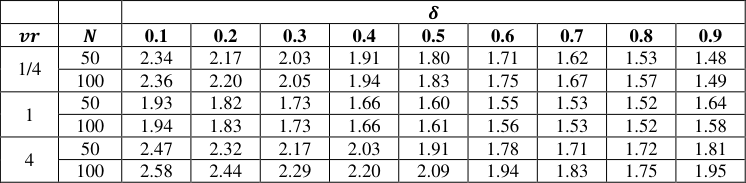 Table 1
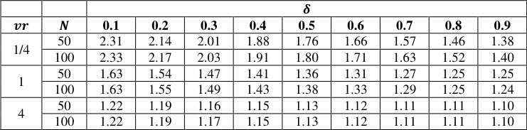 Table 2
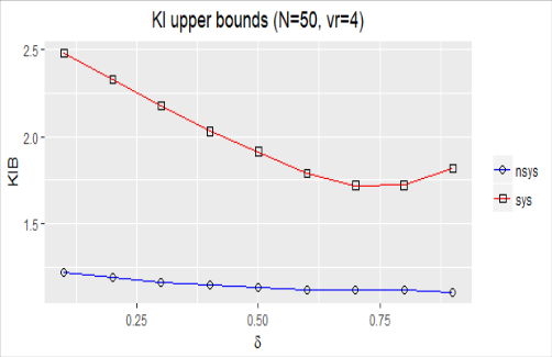 Figure 1
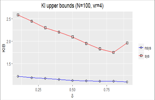 Figure 1
Introduction
used the Kantorovich Inequality Upper Bounds (KIUB) to determine the efficiency of OLS estimator compared to the best linear unbiased estimators for the vector-regressor case in the general linear model. The KIUB for matrix-regressor case including single positive definite matrix is given by Marshall and Olkin (1990) [5] and Baksalary and Puntanen (1991) [1] . Later, the KIUB with two positive definite matrices is presented by Wang and Shao (1992) [6] . In the panel data context Liu and Neudecker (1997) [3] present the new multivariate versions of the KIUB with two positive definite matrices for Minimum distance (MD) estimator, Generalized Method of Moments (GMM) estimator and Weighted Least Square (WLS) estimator and are applied to compare the inefficient and efficient estimators. Windmeijer (2000) [7] has used the approach of Liu and Neudecker (1997) [3] and computed KIUB using the weight matrices of one-step and its respective two-step system GMM estimator, where the weight matrix of two-step system GMM estimator is computed based on the asymptotic properties (𝜓 𝑠 = 𝑝𝑙𝑖𝑚 𝑊 𝑠2 -1 , where 𝑊 𝑠2 -1 is the weight matrix of one-step system GMM estimator) and it is observed that KIUB values increases for the case 𝑇 ≥ 4. In this paper, the KIUB are used to obtain the efficiency loss of one-step system and new onestep system GMM estimators compared to their respective efficient two-step estimators. The KIUB are computed for the one-step system GMM estimator with conventional weight matrix and the new one-step system GMM estimator with new weight matrix. The weight matrix of two-step system GMM estimator is computed without using the asymptotic property (𝜓 𝑠 = 𝑊 𝑠2 -1 ). The rest of the paper is as follows. Section 2 provides the AR(1) panel data model, its assumptions, system GMM estimator and New system GMM estimator. Efficiency loss of system and new system GMM estimators is presented in Section 3. Monte Carlo simulation design, results and discussions are given in Section 4. Section 5 presents some concluding remarks.
AR(1) panel data model and assumptions
The first-order autoregressive panel data model is given by, 𝑦 𝑖𝑡 = 𝛿𝑦 𝑖𝑡-1 + 𝑢 𝑖𝑡 , 𝑖 = 1, 2, … , 𝑁; 𝑡 = 2, 3, … , 𝑇.
(1) 𝑢 𝑖𝑡 = 𝜂 𝑖 + 𝑣 𝑖𝑡 Where, 𝜂 𝑖 are individual effects, 𝑣 𝑖𝑡 are idiosyncratic errors, 𝑁 is number of individuals, 𝑇 is time period. The initial value is given by,
Where, 𝑤 𝑖1 = ∑ 𝛿 𝑗 𝑣 𝑖1-𝑗 ∞ 𝑗=0
and independent of 𝜂 𝑖 . It is assumed that, 𝐸(𝜂 𝑖 ) = 𝐸(𝑣 𝑖𝑡 ) = 𝐸(𝜂 𝑖 𝑣 𝑖𝑡 ) = 𝐸(𝑦 𝑖1 𝑣 𝑖𝑡 ) = 0, 𝑖 = 1, 2, … , 𝑁; 𝑡 = 2, 3, … , 𝑇.
𝐸(𝑣 𝑖𝑡 𝑣 𝑖𝑠 ) = 0, 𝑖 = 1, 2, … , 𝑁; 𝑡 ≠ 𝑠.
And 𝑉(𝜂 𝑖 ) = 𝜎 𝜂 2 , 𝑉(𝑣 𝑖𝑡 ) = 𝜎 𝑣 2 , 𝑉(𝑢 𝑖𝑡 ) = 𝜎 𝑢 2 , 𝑖 = 1, 2, … , 𝑁; 𝑡 = 2, 3, … , 𝑇.
System GMM Estimator
Under the above-mentioned assumptions, Blundell and Bond (1998) [2] considered system GMM estimator in which the moment conditions of system GMM estimator are the combination of the moment condition of first-difference and level GMM estimators and is given by,
The one-step system GMM estimator is given by,
Where, s i,-1 ′ is the 1 × 2(T -2) vector (Δy i2 , … , Δy iT-1 , y i2 , … , y iT-1 ), s i ′ is the 1 × 2(T -2) vector (Δy i3 , … , Δy iT , y i3 , … , y iT ), s -1 and 𝑠 are stacked across individuals.
matrix with 2's on the main diagonal, -1's on the first subdiagonals and zeros otherwise and
The efficient two-step system GMM estimator is based on the following weight matrix:
Where, 𝑢 ̂𝑠𝑖 is a residual obtained from the one-step system GMM estimator 𝛿 ̂1𝑠𝑦𝑠 .
New System GMM Estimator
The new one-step system GMM estimator considers the new weight matrix (W ns1 ), instead of conventional weight matrix (W s1 ) and is given by,
Where, 𝐴 𝑠 = [ 𝐴 𝑑 0 0 𝐴 𝑙 ] with 𝐴 𝑛𝑙 is a (𝑇 -2) × (𝑇 -2) matrix with 𝜎 𝑢 2 on the main diagonal and 𝜎 𝜂 2 otherwise.
The new two-step system GMM estimator is based on the following weight matrix:
where, 𝑢 ̂𝑛𝑠𝑖 is a residual obtained from the new one-step system GMM estimator.
Efficiency Comparison
To detect which initial weight matrix is to be used to obtain the efficient one-step system GMM estimator, without calculating its variances, the KIUBs are calculated to compare the efficiency difference between the one-step and two-step system GMM estimators.
Efficiency comparison of the one-step system GMM estimator compared to its efficient two-step estimator
Expression for the efficiency comparison between one-step system GMM estimator and its efficient two-step estimator is obtained using the initial weight matrix 𝑊 𝑠1 , which is similar to the expression derived by Liu and Neudecker (1997) [3] and is given by,
) + (T -2). The twostep estimator is asymptotically efficient but not the one-step estimator, since ψ s is based on the one-step estimator, we do not calculate it by using asymptotic property (ψ s -1 = plim N→∞ W s2 ). Now ψ s is given by, Further,
Now, the matrix B = ψ s W s1 is given by, 2 3
𝐸(Δ𝑢 ̂𝑖3 Δ𝑢 ̂𝑖4 ) + 2𝐸(Δ𝑢 ̂𝑖4 ) Now, compute the eigen values of matrix 𝐵 and substitute in the expression
, which is the required KIUB.
Efficiency comparison of the new one-step system GMM estimator compared to its efficient two-step estimator
Expression for the efficiency comparison between new one-step system GMM estimator and its efficient two-step estimator is obtained using the initial weight matrix W ns1 is derived and is given by,
Where, λ B n1 ≥ ⋯ ≥ λ B nm are the eigenvalues of the matrix ψ ns W ns1 . Now ψ s is given by, Further,
Now, the matrix 𝐵 𝑛 = 𝜓 𝑛𝑠 𝑊 𝑛𝑠1 is given by, , 1, 4} and the results are based on 10000 replications. Table 1 and 2 provides the KIUBs of the one-step system GMM estimator (SYS) with the initial weight matrix 𝑊 𝑠1 and the new one-step system GMM estimator (NSYS) with the new initial weight matrix 𝑊 𝑛𝑠1 respectively. Figure 1 presents the KIUB values of SYS and NSYS compared to their respective two-step system GMM estimators.
| — | — | 𝜹 | — | — | — | — | — | — | — | — |
|---|---|---|---|---|---|---|---|---|---|---|
| 𝒗𝒓 | 𝑵 | 0.1 | 0.2 | 0.3 | 0.4 | 0.5 | 0.6 | 0.7 | 0.8 | 0.9 |
| 1/4 | 50 | 2.34 | 2.17 | 2.03 | 1.91 | 1.80 | 1.71 | 1.62 | 1.53 | 1.48 |
| 100 | 2.36 | 2.20 | 2.05 | 1.94 | 1.83 | 1.75 | 1.67 | 1.57 | 1.49 | |
| 1 | 50 | 1.93 | 1.82 | 1.73 | 1.66 | 1.60 | 1.55 | 1.53 | 1.52 | 1.64 |
| 100 | 1.94 | 1.83 | 1.73 | 1.66 | 1.61 | 1.56 | 1.53 | 1.52 | 1.58 | |
| 4 | 50 | 2.47 | 2.32 | 2.17 | 2.03 | 1.91 | 1.78 | 1.71 | 1.72 | 1.81 |
| 100 | 2.58 | 2.44 | 2.29 | 2.20 | 2.09 | 1.94 | 1.83 | 1.75 | 1.95 |
Table text extracted from the original PDF; superscript letters are shown inline. The original table image is below.
View original table image
Results and Discussion
From Table 1 it is observed that, when 𝑣𝑟 = 1 (𝑣𝑟 = variance ratio i.e., 𝑣𝑟 = σ η 2 σ v 2 ), the KIUB values of SYS is almost same for both 𝑁 = 50 and 100. When 𝑣𝑟 is less than or greater than 1, the KIUB values of SYS differs for both 𝑁 = 50 and 100. Same can be observed in the case of NSYS (Table 2). From Table 2 it is also observed that as 𝑣𝑟 increases KIUB decreases. From both Table 1 and 2 it is observed that for different values of 𝑣𝑟, KIUB decreases with 𝛿. For all the values of 𝛿, 𝑣𝑟 and 𝑁, the KIUB values of NSYS are lesser than the values of SYS.
| — | — | 𝜹 | — | — | — | — | — | — | — | — |
|---|---|---|---|---|---|---|---|---|---|---|
| 𝒗𝒓 | 𝑵 | 0.1 | 0.2 | 0.3 | 0.4 | 0.5 | 0.6 | 0.7 | 0.8 | 0.9 |
| 1/4 | 50 | 2.31 | 2.14 | 2.01 | 1.88 | 1.76 | 1.66 | 1.57 | 1.46 | 1.38 |
| 100 | 2.33 | 2.17 | 2.03 | 1.91 | 1.80 | 1.71 | 1.63 | 1.52 | 1.40 | |
| 1 | 50 | 1.63 | 1.54 | 1.47 | 1.41 | 1.36 | 1.31 | 1.27 | 1.25 | 1.25 |
| 100 | 1.63 | 1.55 | 1.49 | 1.43 | 1.38 | 1.33 | 1.29 | 1.25 | 1.24 | |
| 4 | 50 | 1.22 | 1.19 | 1.16 | 1.15 | 1.13 | 1.12 | 1.11 | 1.11 | 1.10 |
| 100 | 1.22 | 1.19 | 1.17 | 1.15 | 1.13 | 1.12 | 1.11 | 1.11 | 1.10 |
Table text extracted from the original PDF; superscript letters are shown inline. The original table image is below.
View original table image
The one-step GMM estimator is said to be efficient when the KIUB value is near to one. From the above two table it is found that the KIUB values of NSYS estimator is near to 1 than the KIUB values of SYS estimator. When 𝑣𝑟 = 4, 𝛿 = 0.5 and𝑁 = 100, the KIUB value of NSYS is 1.13215, indicating that the one-step NSYS estimator is 13% inefficient than its two-step NSYS estimator. Figure 1 shows that as 𝑣𝑟 increases the difference between KIUB of SYS and NSYS increases and the same pattern is observed for both 𝑁 = 50 and 100. For all the values of 𝛿, 𝑣𝑟 and 𝑁, the NSYS has a minimum KIUB value than the SYS.
Conclusion
From the earlier study, it is known that the system GMM estimator is efficient for the autoregressive panel data model than the other GMM estimators and also known that the two-step estimator is efficient than the one-step estimator. In the above study, we computed the KIUBs for one-step system and new system GMM estimators compared to their respective efficient two-step GMM estimators. It is observed that the KIUB values of NSYS estimator is near to one than the SYS estimator, which means one-step NSYS estimator is efficient than the one-step SYS estimator. We conclude that it is better to use the new weight matrix 𝑊 𝑛𝑠1 to compute one-step system GMM estimator instead of using conventional weight matrix 𝑊 𝑠1 .
References
7 in the original paper- Baksalary JK, Puntanen S. Generalized matrix versions of the Cauchy-Schwarz and Kantorovich inequalities, Aequationes Math. 1991; 41:103-110.
- Blundell R, Bond S. Initial Conditions and Moment Restrictions in Dynamic Panel Data Models. Journal of Econometrics. 1998; 87:115-143.
- Liu S, Neudecker H. Kantorovich inequalities and efficiency comparisons for several classes of estimators in linear models. Statistica Neerlandica. 1997; 55:345-355.
- Magness TA, McGuire JB. Comparison of least squares and minimum variance estimates of regression parameters. The Annals of Mathematical Statistics. 1962; 33:462-470.
- Marshall AW, Olkin I. Matrix versions of the Cauchy and Kantorovich inequalities, Aequationes Mathematicae. 1990; 40:8993.
- Wang SG, Shao J. Constrained Kantorovich inequalities and relative efficiency of least squares. Journal of Multivariate Analysis. 1992; 42:284-298.
- Windmeijer F. Efficiency comparisons for a system GMM estimator in dynamic panel data models. In Innovations in Multivariate Statistical Analysis. 2000, 175-184.