
Research article · 2026 · Full text
International Journal of Geography Geology and EnvironmentExplainable artificial intelligence for climate change impact assessment using multi-temporal geospatial data
Volume 8(9) · Pages 26–34 · DOI: 10.22271/27067483.2026.v8.i9a.862 ↗
Research areasClimate Change and Environmental ImpactUrban Heat Island MitigationRemote-Sensing Image Classification
Abstract
Author-writtenClimate change increasingly affects urban environmental systems through changes in Temperature, vegetation, water availability, and land-surface conditions. Previous studies have assessed individual or multiple climate hazards using remote sensing and machine learning; however, limited integration of compound climate impacts, fine-scale spatial assessment, temporal variability, and model interpretability remains a research gap. This study aimed to develop an integrated and explainable framework for assessing climate-change impacts in Lucknow. Landsat 8-9 Operational Land Imager (OLI)/ Thermal Infrared Sensor (TIRS) and ERA5-Land datasets were preprocessed and spatially harmonized, followed by climate-impact indicator extraction, multi-temporal feature engineering, Categorical Boosting (CatBoost)-based modelling, Climate Change Impact Index (CCII) development, SHapley Additive exPlanations (SHAP)-based interpretation, and spatio-temporal assessment. The framework assessed four dimensions: heat impact, vegetation stress, water stress, and land-surface change. The CatBoost model achieved Coefficient of Determination (R²) values ranging from 0.89 to 0.94 and Root Mean Square Error (RMSE) values ranging from 0.044 to 0.056 across these dimensions. Overall, the proposed framework effectively integrated prediction, explainability, and spatial assessment, providing a comprehensive basis for climate-impact monitoring and supporting future applications with higher-resolution datasets and advanced spatio-temporal modelling approaches.
Summary
Source-checkedPlain-language reading of the full paper, prepared with AI and checked against the text. Each point links to the authors' own words.
Why it matters
- Climate change is impacting urban environments by altering temperature, vegetation, water availability, and land-surface conditions. View evidence ↗
- Current research lacks sufficient integration of compound climate impacts, fine-scale spatial analysis, and interpretable models. View evidence ↗
The question
- The study aims to create an integrated and explainable framework to assess the impacts of climate change in Lucknow, India. View evidence ↗
What they did
- The researchers used Landsat 8-9 OLI/TIRS satellite imagery and ERA5-Land climate data as secondary data sources. View evidence ↗
- The assessment framework focused on four specific dimensions: heat impact, vegetation stress, water stress, and land-surface change. View evidence ↗
- The methodology employed CatBoost for modeling, developed a Climate Change Impact Index (CCII), and used SHAP for model interpretation. View evidence ↗
What they found
- All four climate-impact indicators showed an increasing trend from 2013 to 2024, with the Heat Impact Index rising from 0.42 to 0.72. View evidence ↗
- The most substantial temporal change occurred in the historical-to-recent change feature, which increased from 0.08 in 2013 to 0.42 in 2024. View evidence ↗
- The overall Climate Change Impact Index (CCII) increased from 0.35 in 2013 to 0.66 in 2024. View evidence ↗
- Spatially, the CCII varied from a minimum of 0.31 to a maximum of 0.66 across the study area grid. View evidence ↗
- SHAP analysis identified Temperature, Precipitation, and the Vegetation Index as significant features influencing the model's predictions. View evidence ↗
- The CatBoost model demonstrated high predictive performance, with R² values between 0.89 and 0.94 and RMSE values between 0.044 and 0.056 across all dimensions. View evidence ↗
What it means
- The authors conclude that their framework effectively integrates prediction and explainability, offering a comprehensive tool for monitoring climate impacts. View evidence ↗
- The authors suggest that future work should incorporate higher-resolution datasets and additional climate indicators to extend the framework. View evidence ↗
Visual summary
3 visualsIllustrations explain the paper; charts are replotted from the paper's own table values.
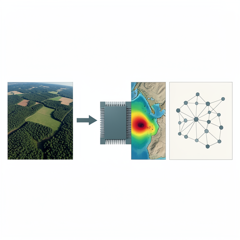
Framework Workflow
AI-generated conceptual illustration (Satellite-viewed landscape and a computer processor). It explains the idea and does not show study data.
View source evidence ↗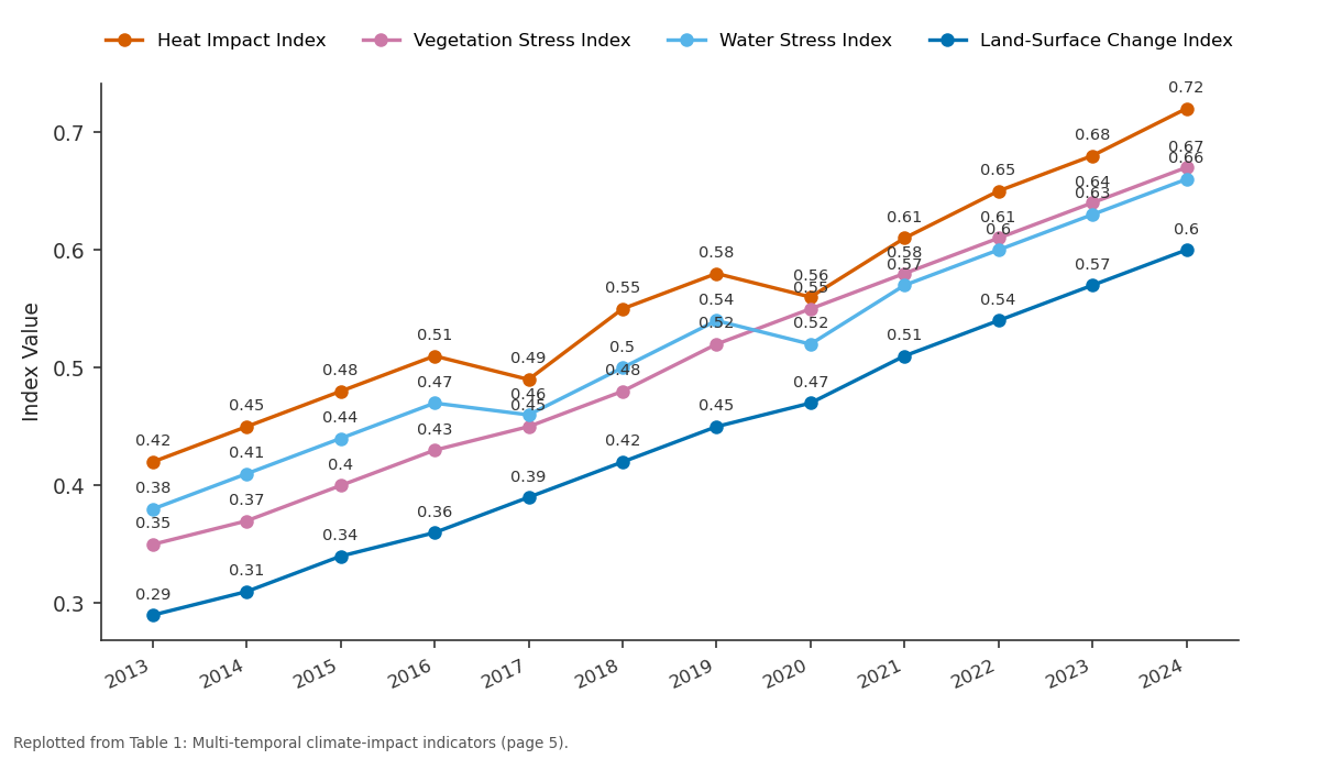
Heat Impact Index and Vegetation Stress Index and more: 2013 vs 2014 vs 2015 vs 2016 vs 2017
Replotted from Table 1 (page 5) of the original paper. Every bar is the paper's own table value.
View source evidence ↗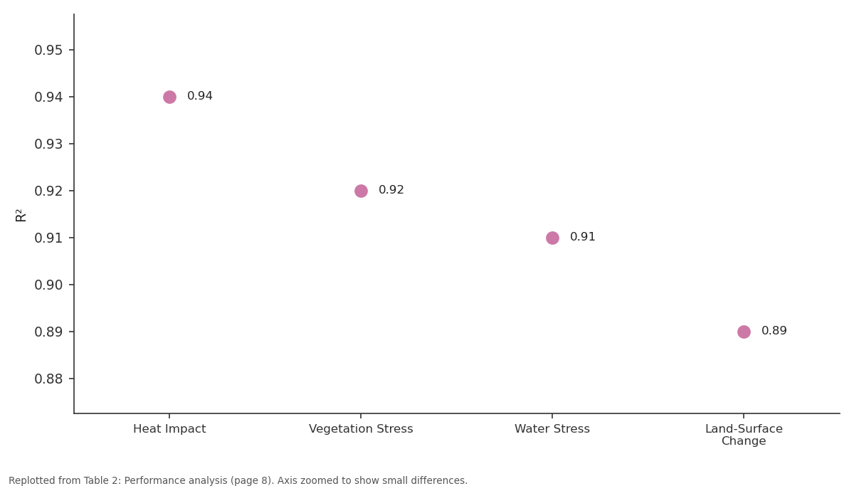
R²: Heat Impact vs Vegetation Stress vs Water Stress vs Land-Surface Change
Replotted from Table 2 (page 8) of the original paper. Every bar is the paper's own table value.
View source evidence ↗Figures & tables
From the original paper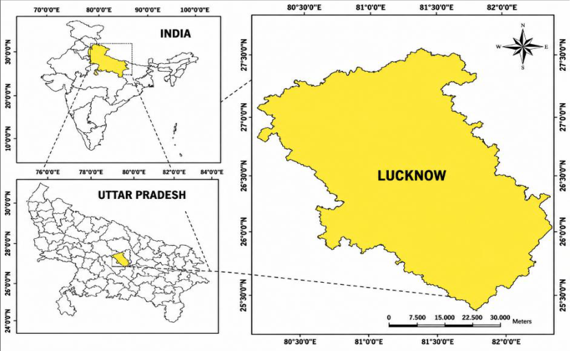 Figure 1
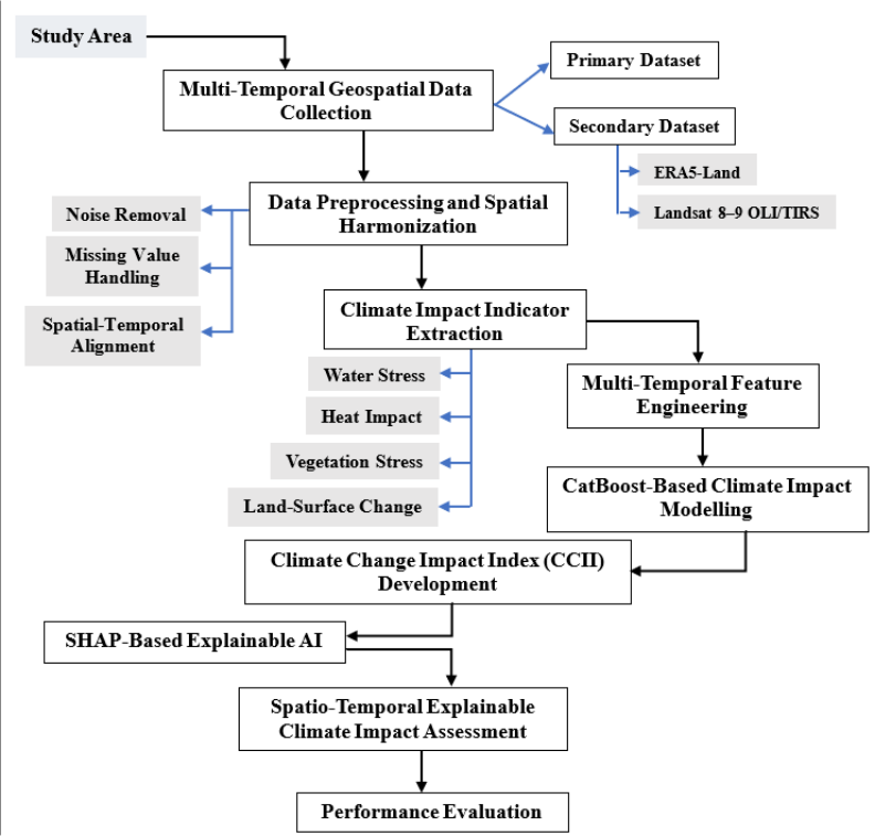 Figure 2
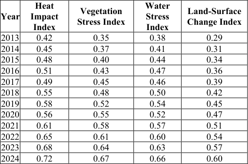 Table 1
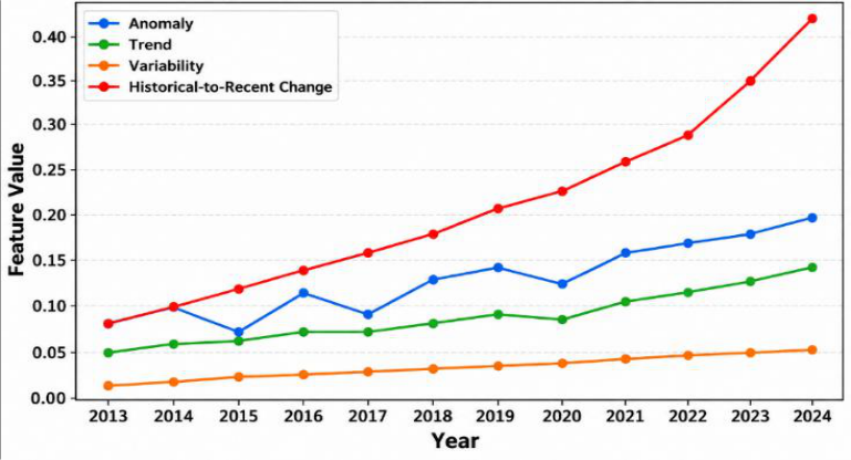 Figure 3
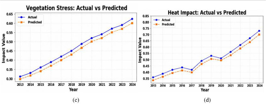 Figure 4
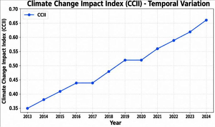 Figure 5
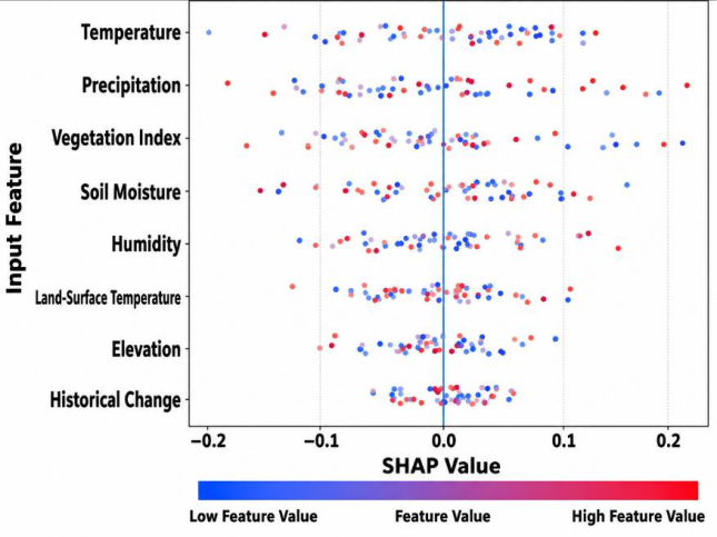 Figure 6
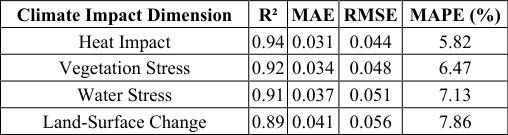 Table 2
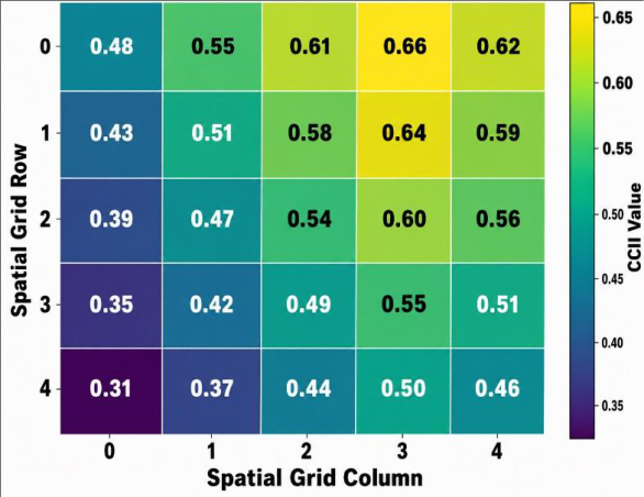 Figure 7
Introduction
The effects of climate change are bringing changes in environmental circumstances with increased exposure of natural and human-made systems to various effects of climate change such as heat, drought, flood, water stress, deterioration of vegetation, and others [1] . These changes are heterogeneous in nature and differ greatly in terms of time; hence, their assessment relies heavily on data that can describe the changes geographically and temporally. Multi-temporal geospatial technologies have proven to be an excellent way of observing these changes by virtue of the use of satellite imagery, climatic data, land cover, and other types of spatial data [2,3] . Data collected over different times makes it possible to analyze environmental changes related to climate change. However, there are difficulties associated with analyzing multitemporal geospatial data due to its voluminous nature and characteristics [4][5][6] . Artificial Intelligence (AI), machine learning, and Geospatial Artificial Intelligence (GeoAI) have been increasingly utilized for evaluating complex interactions of climatic and environmental phenomena, hazards, the impact of drought, flood vulnerability, land use, and climate adaptation [7,8] . Various works have utilized Light Gradient Boosting Machine (LightGBM), Extreme Gradient Boosting (XGBoost), Random Forest (RF), and Analytical Hierarchy Process (AHP) for spatial risk assessment; Explainable Artificial Intelligence (XAI) methods like SHAP have been used for assessing contributions of individual features to model results [9] . However, the existing approaches do not address compound and synergetic effects of climate-based hazards. Fine-scale assessments as well as socioeconomic vulnerability have not been sufficiently addressed [10] . In addition to that, the use of certain time windows as well as geographically confined case studies limited the evaluation of temporal dynamics and the general applicability of models developed [11] . It is thus evident that there is a need of framework allowing temporal geospatial data to be combined with prediction and interpretability.
To overcome these limitations, this research suggests an explainable AI framework for assessing the impact of climate change at multiple temporal scales in Lucknow based on the integration of geospatial and climate data. Landsat 8-9 OLI/TIRS and ERA5-Land data were combined to construct four dimensions of climate-impact effects, namely heat effect, vegetation stress, water stress, and land surface changes. Temporal feature engineering was done to extract anomaly, trend, variability, and historical-to-recent change information from the dataset, and CatBoost was used to model the association of features with the outcome of climate-impact effects. SHAP further enables the interpretation of feature importance and identification of factors influencing the prediction results. The novelty of the study is the combination of multitemporal geospatial data analysis, climate impact indicator extraction, temporal feature engineering, CatBoost machine learning algorithm application, CCII construction, and SHAP explainability technique within one climate change impact assessment model. The purpose of this study is the assessment of climate impacts during different time periods, estimation of their spatial and temporal dynamics, identification of influential climatic and environmental factors, and providing explainable climate impact predictions. The key contributions of this study are:
• Proposed an explainable AI-based approach for assessing impacts of climate change through multiple time periods in Lucknow using geospatial and climatic data.
Literature Review
This section reviews and summarizes previous studies related to climate-change impact assessment, multi-temporal geospatial analysis, machine learning-based modelling, and XAI for environmental assessment. Singh et al. (2026) [12] introduced LightGBM with SHAP to assess Delhi's multi-hazard risk using 22 predictors. The model achieved R² of 0.98 and Mean Absolute Error (MAE) of 0.01 across spatial validation folds, demonstrating predictive performance for regional multi-hazard assessment and risk characterization. Yao et al. (2026) [13] developed XGBoost with SHAP to assess multi-hazard risk and land-use effects in Ningbo.
Results showed that green/forest land dominated risk patterns, while built-up and green/forest land thresholds were identified at 20.0% and 2.0%, respectively, regionwide. Bovkir (2026) [14] employed GeoAI with SHAP to assess climate adaptation needs across 1, 187 European regions. The Climate Change Adaptation Index (CCAI) used 44 indicators and identified heat stress, precipitation, and renewable energy as important contributors to regional adaptation needs.
Chauhan and Ngangom (2026) [15] applied an AHP-based geospatial approach to assess four climate-induced hazards in Ladakh. The resulting maps achieved accuracies of 75%, 80%, 88%, and 90% for floods, landslides, snow avalanches, and droughts, respectively, overall. Hrast Essenfelder et al. (2025) [16] introduced an expertdriven XAI model using XGBoost to detect agricultural climate hazards. The model provided hazard detection, uncertainty estimation, and drivers, supporting risk management and adaptation through understanding of climate extremes. Sanderson et al. (2023) [17] developed XFIMNet, an explainable encoder-decoder model using multispectral and Synthetic Aperture Radar (SAR) imagery for flood mapping. The model achieved Intersection over Union (IoU) values of 0.5862 and 0.7031 using Sentinel-1 and Sentinel-2 imagery, respectively, demonstrating flood detection.
Zhang et al. (2023) [18] utilized an explainable XGBoost-SHAP pipeline to predict drought impacts and interpret climatic drivers. The model achieved F2 scores of 0.883 nationally and 0.942 at the state level, providing interpretable insights into climatic factors influencing drought impacts. Zhang et al. (2023) [19] employed ML models, including RF, to assess multi-hazard risk and social vulnerability in Idaho. RF performed best across hazard and vulnerability datasets, while 15.88% of cities were classified as high-risk multihazard and vulnerable.
Research Gaps
Although current literature has shown some advances in the field of multi-hazard assessment, there are still many drawbacks that should be addressed. Current research has shown many cases of single or multiple hazard assessment without taking into account their compounding and synergies effects, thus not enabling proper risk characterization [12,16,19] . In most of the cases, regional-scale assessment was carried out, and fine-resolution spatial analysis as well as socioeconomic vulnerability were not taken into account properly [13,15,17] . There are also problems with uncertainty calibration and temporal generalization since many studies are conducted under specific conditions [15,16] .
Research Methodology
This section provides an overview of the study area, data sources, techniques, and proposed research framework used in the study.
Study Area
The experiment was performed in Lucknow, Uttar Pradesh, India, which is situated at around 26°51′ N latitude and 80°57′ E longitude, with an elevation of around 123 m above mean sea level and an area covering approximately 350 km². The climate of the city is humid subtropical with precipitation of about 1, 000 mm per year. The mentioned features make Lucknow appropriate for studying the variability of heat effect, vegetation stress, water stress, and land surface changes with multi-temporal geospatial data.
The geographical location of Lucknow, Uttar Pradesh, India is depicted in Figure 1. Study area and spatial analysis grid of Lucknow [20] Data Collection Primary and secondary sources were used in the study to assess the impact of climate change on Lucknow through multiple periods. Primary sources consisted of the spatial boundary of Lucknow, whereas secondary sources were Landsat 8-9 OLI/TIRS Collection 2 Level 2 images and ERA5-Land climate data.
Primary Data
The primary data consisted of the Lucknow spatial boundary data obtained from the Lucknow Remote Sensing Application Centre (LRSAC). The boundary was used to delineate the study area and provide a common spatial framework for integrating the multi-temporal datasets.
Secondary Data Landsat 8-9 OLI/TIRS
The satellite images were obtained from EarthExplorer, which is a US Geological Survey (USGS) portal. The Landsat 8 and Landsat 9 images provide surface reflectance and land surface temperature data at 30-meter spatial resolution. The data have been utilized to obtain indicators of heat impact, vegetation stress, water stress, and landsurface change. The Landsat 8 images are available since 2013, whereas Landsat 9 images are available since 2022 [21] .
ERA5-Land
The ERA5-Land data [22] were sourced from the Copernicus Climate Data Store. This dataset has climate and land surface variables such as Temperature, precipitation, and soil water data dating back from 1950 onwards. The dataset has a spatial resolution of about 9 kilometers. The variables were used as climate predictors for further analysis.
Techniques Used
This section presents the CatBoost, CCII, and SHAP techniques used for climate impact modelling and interpretation.
CatBoost
CatBoost is a gradient-boosting machine learning technique that establishes the relation between multi-temporal climatic, remote-sensing, geospatial, and temporal variables and climatic impact outcomes [23] . CatBoost constructs an ensemble of decision trees such that each tree constructed minimizes the prediction error of the ensemble constructed previously. The general form of the prediction function is given by:
Where represents the predicted climate-impact value for observation , represents the input features, denotes the number of boosting iterations, and represents the decision tree. The objective function is expressed as:
Where represents the prediction loss, and controls the complexity of the individual trees. In this study, CatBoost models the relationships between multi-temporal input features and the four climate-impact dimensions: heat impact, vegetation stress, water stress, and land-surface change.
Climate Change Impact Index
The CCII is developed by integrating the four standardized climate-impact dimensions: heat impact, vegetation stress, water stress, and land-surface change. The index provides an overall measure of climate-impact intensity for different spatial and temporal units. It is calculated as:
Where represents the Climate Change Impact Index for observation , while , and represent the standardized heat impact, vegetation stress, water stress, and land-surface change values, respectively.
SHAP
SHAP is an XAI technique that interprets CatBoost predictions by quantifying the contribution of individual input features to each prediction. The SHAP explanation is expressed as:
Where denotes the model prediction, denotes the expected model output, stands for the number of input features, and characterizes the contribution of feature . The SHAP value for feature is formulated as: (5) Where symbolizes a subset of features, denotes the complete set of features, and signifies the model prediction using the features in subset . In this study, SHAP identifies the relative importance and positive or negative contribution of climate, remote-sensing, geospatial, and temporal features to the climate-impact predictions.
Proposed Methodology
The proposed methodology begins with study area selection and the acquisition of multi-temporal geospatial datasets for Lucknow. The complete process flowchart of the methodological framework is depicted in Figure 2 through the methodology architecture. The acquired datasets are preprocessed and harmonized spatially, which involves processing for handling missing values, noise elimination, and spatiotemporal normalization. Climate impact indicators are calculated for heat impact, vegetation stress, water stress, and land surface changes. At the same time, multitemporal feature engineering is done to extract the anomaly, trend, variation, and change features. These features are utilized in climate impact modeling using the CatBoost algorithm, and then all four dimensions of the impact are combined to formulate the CCII. Feature contribution interpretation is performed through SHAP, followed by spatiotemporal climate impact assessment to discover climate impact patterns and changing factors.
Results and Analysis
In this section, the findings of the climate-change impact assessment framework proposed for Lucknow are presented. The CatBoost model was configured with the following hyperparameters: 500 iterations, a learning rate of 0.05, a tree depth of 6, and a random seed of 42. The proposed model was evaluated using the following metrics:
Where represents the actual climate-impact value for the -th observation, represents the corresponding predicted value obtained from the CatBoost model, denotes the mean of the actual values, represents the total number of observations, and denotes the index of each observation, ranging from to . The framework uses the Lucknow spatial boundary dataset as primary data and Landsat 8-9 OLI/TIRS satellite imagery and ERA5-Land climate datasets as secondary datasets. The acquired data were preprocessed through missing-value treatment, noise reduction, cloud-contaminated observation processing, and spatio-temporal harmonization. Once the preprocessing and spatial-temporal alignment of the collected datasets were completed, the four climate impact indices were calculated as measures of the main aspects of environmental changes associated with the climate of Lucknow. These four climate impact indices are the annual values of the Heat Impact Index, Vegetation Stress Index, Water Stress Index, and Land-Surface Change Index. The annual variations of these four indices over the study period are presented in Table 1. They exhibit an increasing trend over time throughout the entire study period. Based on the indicators related to the impact of climate on the environment, multi-temporal features were derived in order to represent their behavior in time over the entire study period. Figure 3 The analysis of the CCII index from the point of view of the CatBoost modeling results demonstrated a positive trend for this parameter throughout the study period. As can be seen in Figure 5, the CCII index rose from 0.35 in 2013 to 0.66 in 2024, with a stable value of 0.44 from 2016 to 2017 and 0.52 from 2019 to 2020 and then rose to 0.66 in 2024. Based on the CCII findings, SHAP analysis was carried out for the interpretation of the contributions of the input features to the CatBoost model. According to Figure 6, the SHAP value of Temperature was found to be broadly distributed between -0.20 and 0.14, whereas that of Precipitation and Vegetation Index were broadly distributed between -0.18 and 0.22, and -0.16 and 0.21, respectively.
| Year | Heat Impact Index | Vegetation Stress Index | Water Stress Index | Land-Surface Change Index |
|---|---|---|---|---|
| 2013 | 0.42 | 0.35 | 0.38 | 0.29 |
| 2014 | 0.45 | 0.37 | 0.41 | 0.31 |
| 2015 | 0.48 | 0.40 | 0.44 | 0.34 |
| 2016 | 0.51 | 0.43 | 0.47 | 0.36 |
| 2017 | 0.49 | 0.45 | 0.46 | 0.39 |
| 2018 | 0.55 | 0.48 | 0.50 | 0.42 |
| 2019 | 0.58 | 0.52 | 0.54 | 0.45 |
| 2020 | 0.56 | 0.55 | 0.52 | 0.47 |
| 2021 | 0.61 | 0.58 | 0.57 | 0.51 |
| 2022 | 0.65 | 0.61 | 0.60 | 0.54 |
| 2023 | 0.68 | 0.64 | 0.63 | 0.57 |
| 2024 | 0.72 | 0.67 | 0.66 | 0.60 |
Table text extracted from the original PDF; superscript letters are shown inline. The original table image is below.
View original table image
On the other hand, the values for Soil Moisture were found to be broadly distributed between -0.15 and 0.12, whereas those for Humidity and Land Surface Temperature had comparatively smaller ranges. Elevation and Historical Change had the lowest SHAP value ranges. Using the interpretative analysis of SHAP, the spatial pattern of CCII was analysed in the established spatial grid.
As can be seen in Figure 7, the CCII ranged from 0.31 to 0.66, where the minimum CCII was 0.31 in Grid Row 4, Column 0, whereas the maximum value was 0.66 in Grid Row 0, Column 3. The high CCII was clustered in the upper-right portion of the grid, whereas low CCII was found in the lower-left portion of the grid.
Figures and tables from the paper
| Climate Impact Dimension | R² | MAE | RMSE | MAPE (%) |
|---|---|---|---|---|
| Heat Impact | 0.94 | 0.031 | 0.044 | 5.82 |
| Vegetation Stress | 0.92 | 0.034 | 0.048 | 6.47 |
| Water Stress | 0.91 | 0.037 | 0.051 | 7.13 |
| Land-Surface Change | 0.89 | 0.041 | 0.056 | 7.86 |
Table text extracted from the original PDF; superscript letters are shown inline. The original table image is below.
View original table image
References
21 in the original paper- Moldavan L, Pimenowa O, Wasilewski M, Wasilewska N. Sustainable development of agriculture of Ukraine in the context of climate change. Sustainability. 2023;15(13):10517. https://doi.org/10.3390/su151310517
- Bagheri M, Tshireletso T, Ghorashi SA. From multisensor fusion to intelligent geospatial monitoring: emerging architectures for geotechnical hazard assessment. Remote Sens. 2026;18(16):2669. https://doi.org/10.3390/rs18162669
- Vitale A, Lamonaca F. Advancing built-up area monitoring through multi-temporal satellite data fusion and machine learning-based geospatial analysis. Remote Sens. 2025;17(11):1830. https://doi.org/10.3390/rs17111830
- Dritsas E, Trigka M. Remote sensing and geospatial analysis in the big data era: a survey. Remote Sens. 2025;17(3):550. https://doi.org/10.3390/rs17030550
- Kazemi Garajeh M, Salmani B, Zare Naghadehi S, Valipoori Goodarzi H, Khasraei A. An integrated approach of remote sensing and geospatial analysis for modeling and predicting the impacts of climate change on food security. Sci Rep. 2023;13(1):1057. https://doi.org/10.1038/s41598-023-28244-5
- Kasahun M. Quantifying deforestation drivers through multi-temporal LULC analysis and population-forest correlation modeling: a case study of Dara Woreda, Ethiopia. Environ Chall. 2025;19:101163. https://doi.org/10.1016/j.envc.2025.101163
- Rathoure AK. Harnessing artificial intelligence and geospatial technologies for assessing environmental vulnerability and risks. In: Intelligent solutions to evaluate climate change impacts. Hershey: IGI Global Scientific Publishing; 2025. p. 239-256. https://doi.org/10.4018/979-8-3693-5898-6.ch010
- Bovkir R. Linking vulnerability and resilience for climate change adaptation: a GeoAI-integrated assessment across Europe. Ecol Process. 2026;15(1):22. https://doi.org/10.1186/s13717-026-00680.
- Iban MC, Bilgilioglu SS. Snow avalanche susceptibility mapping using novel tree-based machine learning algorithms (XGBoost, NGBoost, and LightGBM) with eXplainable Artificial Intelligence (XAI) approach. Stochastic Environ Res Risk Assess. 2023;37(6):22432270. https://doi.org/10.1007/s00477-023-02392-6
- Khosravi Y, Ouarda TBMJ. Drought risks are projected to increase in the future in central and southern regions of the Middle East. Commun Earth Environ. 2025;6(1):384. https://doi.org/10.1038/s43247-02502359-1
- Wang P, Zheng X, Liu H. Simulation and forecasting models of COVID-19 taking into account spatiotemporal dynamic characteristics: a review. Front Public Health. 2022;10:1033432. https://doi.org/10.3389/fpubh.2022.1033432
- Singh S, Pandey S, Jain AK, Mousa A, Ben Hasher FF, Zhran M. Integrated multi-hazard risk assessment for Delhi with quantile-regressed LightGBM and SHAP interpretation. Land. 2026;15(3):488. https://doi.org/10.3390/land15030488
- Yao Q, An N, Yao Y, An H, Lu H. Explainable machine learning-based assessment of urban climate change risks and driving mechanisms of land-use characteristics in Ningbo. Land. 2026;15(7):1257. https://doi.org/10.3390/land15071257
- Bovkir R. Linking vulnerability and resilience for climate change adaptation: a GeoAI-integrated assessment across Europe. Ecol Process. 2026;15(1):22. https://doi.org/10.1186/s13717-026-00680-x
- Chauhan P, Ngangom M. Spatio-temporal analysis of climate-induced multi-hazards in Ladakh using geospatial techniques. Discover Geosci. 2026;4(1):100. https://doi.org/10.1007/s44288-026-00469-7
- Hrast Essenfelder A, Toreti A, Seguini L. Expert-driven explainable artificial intelligence models can detect multiple climate hazards relevant for agriculture. Commun Earth Environ. 2025;6(1):207. https://doi.org/10.1038/s43247-024-01987-3
- Sanderson J, Mao H, Abdullah MAM, Al-Nima RRO, Woo WL. Optimal fusion of multispectral optical and SAR images for flood inundation mapping through explainable deep learning. Information. 2023;14(12):660. https://doi.org/10.3390/info14120660
- Zhang B, Abu Salem FK, Hayes MJ, Smith KH, Tadesse T, Wardlow BD. Explainable machine learning for the prediction and assessment of complex drought impacts. Sci Total Environ. 2023;898:165509. https://doi.org/10.1016/j.scitotenv.2023.165509
- Zhang T, Wang D, Lu Y. Machine learning-enabled regional multi-hazards risk assessment considering social vulnerability. Sci Rep. 2023;13(1):13405. https://doi.org/10.1038/s41598-023-40159-9
- Maity N, Mishra VN. Urban growth analysis using multi-temporal remote sensing image and landscape metrics for smart city planning of Lucknow District, India. Eng Proc. 2024;82(1):59. https://doi.org/10.3390/ecsa-11-20514
- Li S, Zeng Y, Dong J, Qin Y. An improved CatBoost model for predicting landslide spatial distribution. Eng. 2026;7(5):233. https://doi.org/10.3390/eng7050233