
Research article · 2026 · Full text
International Journal of Geography Geology and EnvironmentAn integrated geospatial–hydrometeorological framework for developing HEC-HMS input datasets in data-constrained river basins: Application to the Tana River Basin, Kenya
Volume 8(8) · Pages 138–145 · DOI: 10.22271/27067483.2026.v8.i8b.856 ↗
Research areasHydrology and Watershed Management StudiesPrecipitation Measurement and AnalysisSoil Moisture and Remote Sensing
Abstract
Author-writtenReliable HEC-HMS modelling depends on spatially consistent, quality-controlled environmental inputs, yet input-data development is often treated as routine preprocessing. This study developed an integrated geospatial–hydrometeorological workflow for preparing model-ready HEC-HMS input datasets in data-constrained basins, using Kenya’s Tana River Basin as a case study. A 30 m SRTM DEM, 10 m ESA WorldCover land-use/land-cover data, Hydrologic Soil Groups, daily rainfall from 33 stations, CHIRPS precipitation, and observed discharge were quality assessed and harmonised to a common spatial framework. Terrain conditioning generated 23 computational sub-basins. Land-cover and soil data were integrated at 30 m resolution to derive a distributed Curve Number (CN) surface and area-weighted sub-basin CN values of 63–83. Of 1,023 expected rainfall station-days, 50 (4.89%) were missing and infilled using CHIRPS estimates. Daily rainfall was then interpolated using inverse distance weighting (IDW; p = 2), evaluated by Leave-One-Out Cross-Validation (LOOCV), and aggregated to sub-basin Mean Areal Precipitation (MAP). Interpolation errors were lowest in the upper and central catchments (MAE 0.25–0.45 mm; RMSE 0.35–0.60 mm) and higher in the lower and eastern basin (MAE 0.60–1.10 mm; RMSE up to 1.50 mm). The resulting terrain, runoff-parameter, meteorological, and hydrometric datasets form a traceable model-ready database. The contribution lies in an auditable, transferable input-development architecture that links quality assurance, spatial harmonisation, distributed parameter derivation, rainfall validation, and hydrological aggregation before model implementation.
Summary
Source-checkedPlain-language reading of the full paper, prepared with AI and checked against the text. Each point links to the authors' own words.
Why it matters
- Flood risk in developing regions is exacerbated by climate change and land-use shifts, but risk reduction is hindered by poor hydrometeorological monitoring. View evidence ↗
- The reliability of hydrological models like HEC-HMS depends heavily on the quality and spatial alignment of input data, not just the model's calibration. View evidence ↗
- In data-constrained basins, input data often come from diverse sources with inconsistent coordinate systems, resolutions, and quality controls. View evidence ↗
The question
- The study aims to create a transferable framework to quality-assess, harmonise, and derive model-ready terrain, runoff, and rainfall datasets for semi-distributed hydrological modelling. View evidence ↗
What they did
- Terrain conditioning using a 30 m DEM in ArcGIS Pro 3.4 was used to delineate the watershed into 23 computational sub-basins. View evidence ↗
- Runoff parameters were derived using the SCS Curve Number (CN) method under AMC II conditions, with sub-basin values calculated via area-weighted aggregation. View evidence ↗
- Daily rainfall from 33 stations was interpolated using Inverse Distance Weighting (IDW, p=2) and validated using Leave-One-Out Cross-Validation (LOOCV). View evidence ↗
What they found
- The rainfall dataset had a 4.89% missing data rate (50 out of 1,023 station-days), which was corrected using CHIRPS estimates. View evidence ↗
- Area-weighted Curve Number (CN) values for the sub-basins ranged from 63 (SB2) to 83 (SB20), reflecting hydrological variability across the basin. View evidence ↗
- Rainfall interpolation was most accurate in the upper and central catchments, with Mean Absolute Error (MAE) between 0.25–0.45 mm and Root Mean Square Error (RMSE) between 0.35–0.60 mm. View evidence ↗
- Mean Areal Precipitation (MAP) varied significantly by sub-basin, notably on 29 March (1.102 to 6.175 mm), showing that basin-wide averages would hide critical spatial differences. View evidence ↗
What it means
- The authors conclude that the framework's value is in its auditable architecture, specifically the principle of deriving variables spatially before aggregating them to preserve environmental heterogeneity. View evidence ↗
- Study limitations include the short one-month test period, uneven station distribution, IDW assumptions, lack of independent CHIRPS validation, and potential DEM resolution issues in low-relief areas. View evidence ↗
Visual summary
1 visualsIllustrations explain the paper; they do not show study data.
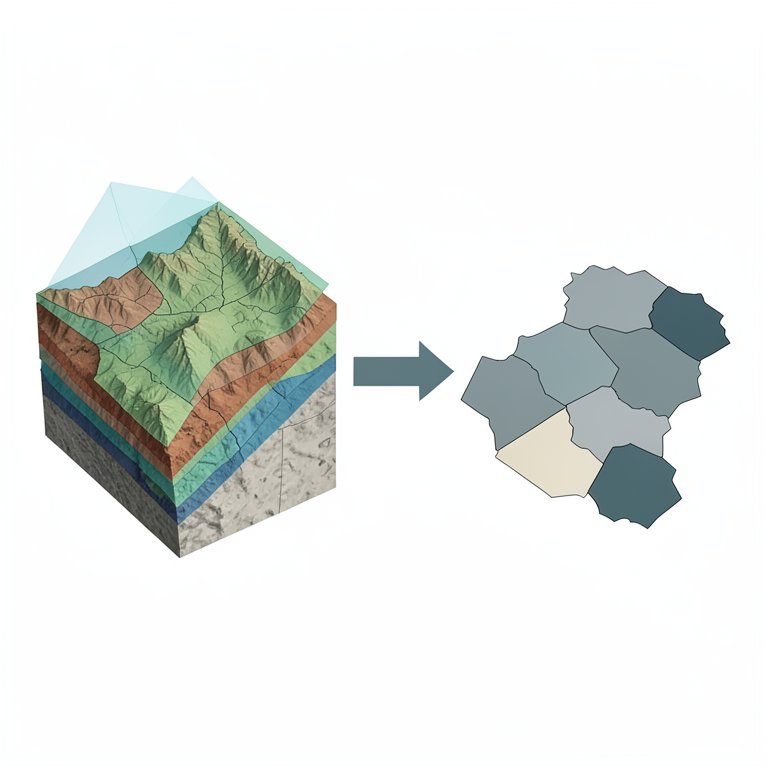
Spatial-to-Hydrological Aggregation Concept
AI-generated conceptual illustration (Tana River Basin, Kenya). It explains the idea and does not show study data.
View source evidence ↗Figures & tables
From the original paper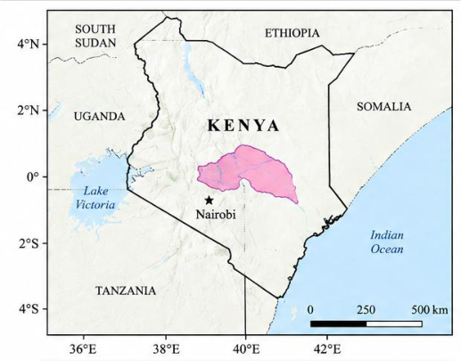 Figure 1
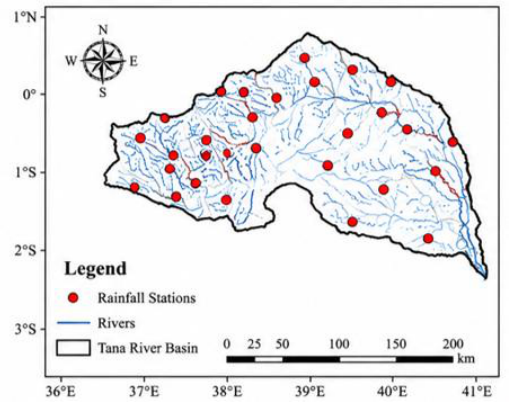 Figure 1
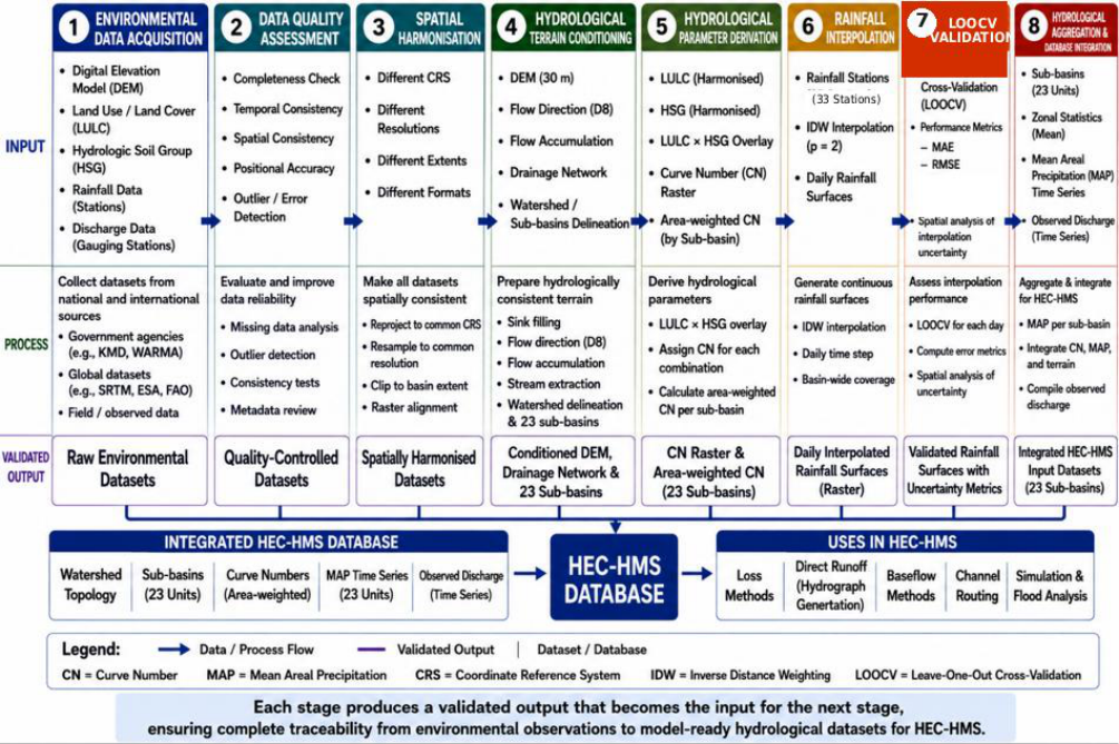 Figure 2
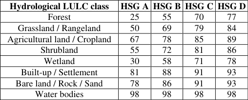 Table 1
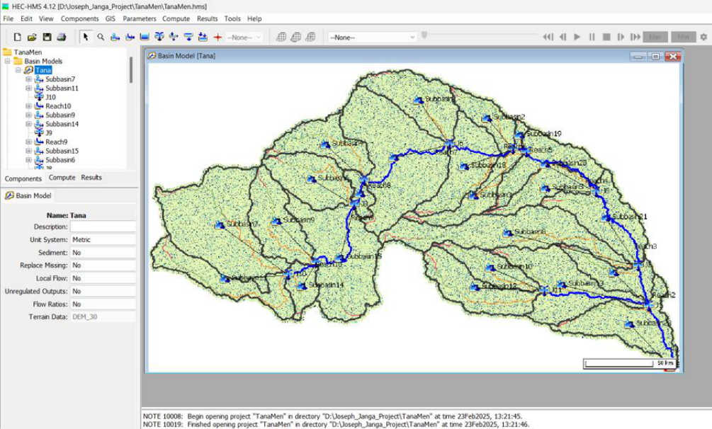 Figure 3
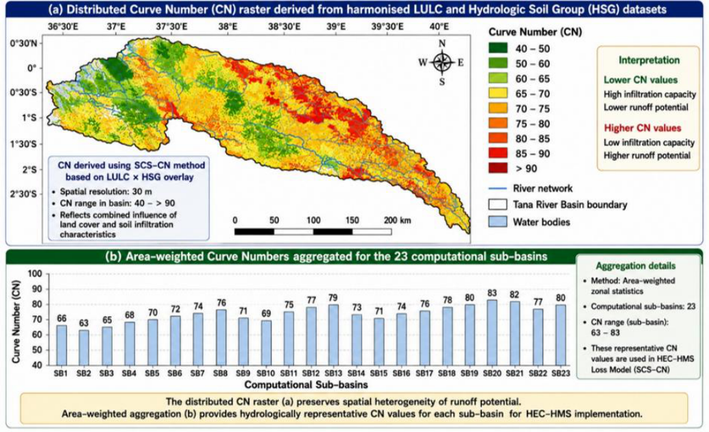 Figure 4
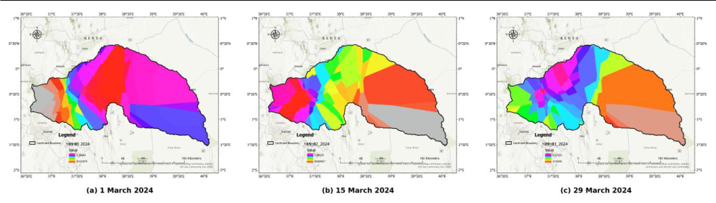 Figure 5
 Table 2
Introduction
Flood risk is shaped by climate variability and change, land-use transformation, population growth, and increasing occupation of flood-prone areas, while weaknesses in hydrometeorological monitoring continue to constrain risk reduction in many developing regions (IPCC, 2022; UNDRR, 2015; WMO, 2021). Reliable hydrological information is therefore central to flood forecasting, disaster-risk reduction, climate adaptation, and waterresources planning. Hydrological models provide a scientific basis for representing rainfall-runoff processes and supporting flood forecasting and watershed management (Beven, 2012; Chow et al., 1988; Maidment, 1993) [2,4,14] . HEC-HMS is widely used because it supports precipitation-runoff transformation, loss methods, routing, continuous simulation, and GIS-based watershed representation (Feldman, 2000; USACE, 2023, 2024). Model reliability, however, depends not only on model structure and calibration but also on the quality, resolution, spatial alignment, and preprocessing of terrain, land-use/land-cover (LULC), soil, rainfall, and discharge inputs. Errors introduced before simulation can propagate through watershed delineation, runoff parameterisation, meteorological forcing, and subsequent flood-risk products (Beven, 2012) [2] . The problem is particularly important in data-constrained basins, where datasets from different institutions and remote-sensing products often differ in coordinate systems, spatial resolution, extent, classification, temporal coverage, and quality-control procedures.
Rainfall presents an additional challenge because gauges are discrete and frequently unevenly distributed; interpolation is therefore necessary, but uncertainty increases where observational support is weak (Goovaerts, 2000; Li & Heap, 2014; Ly et al., 2013) [8,12,13] . Semi-distributed modelling also requires representative sub-basin parameters even though land cover, soils, topography, and rainfall are spatially heterogeneous. A transparent approach is therefore to derive variables at an appropriate spatial resolution, evaluate their quality, and only then aggregate them to model computational units. This study develops and demonstrates an integrated geospatial hydrometeorological framework for producing HEC-HMS input datasets for the Tana River Basin, Kenya. The objectives are to quality-assess and harmonise heterogeneous environmental data; derive terrain, runoffparameter, and rainfall datasets compatible with semidistributed modelling; evaluate interpolated rainfall using Leave-One-Out Cross-Validation (LOOCV); and formulate transferable principles for input-data development. The methodological contribution lies in integrating established procedures into a single auditable workflow rather than proposing a new terrain-processing or rainfall-interpolation algorithm. The study is deliberately limited to input-dataset development and validation rather than HEC-HMS calibration or simulation-performance evaluation.
Materials and Methods
Materials and Methods
Study Area and Data
The framework was applied to the Tana River Basin, Kenya, which covers approximately 126,000 km² and extends from the humid highlands of Mount Kenya and the Aberdare Range through semi-arid lowlands to the Indian Ocean. The basin exhibits pronounced gradients in elevation, rainfall, land cover, soils, and hydrological response, while the rainfall-station network is unevenly distributed. Six datasets were used: a ~30 m SRTM DEM (Farr et al., 2007) [5] ; 10 m ESA WorldCover 2021 v200 LULC (Zanaga et al., 2022) [27] ; Kenya Soil Survey information classified into Hydrologic Soil Groups (HSG A-D); daily rainfall from 33 Kenya Meteorological Department stations for 1-31 March 2024; CHIRPS daily rainfall for gap filling (Funk et al., 2015) [7] ; and Water Resources Authority discharge records retained for subsequent model evaluation. All spatial datasets were referenced to WGS 84 / UTM Zone 37S (EPSG:32737).
Integrated Workflow, Quality Control and Spatial Harmonisation
Dataset development followed eight linked stages: acquisition, quality assessment, spatial harmonisation, terrain conditioning, parameter derivation, rainfall interpolation, LOOCV, and hydrological aggregation/HEC-HMS integration (Figure 2). The DEM was examined for completeness, elevation continuity, voids, and artificial depressions; LULC and HSG data were checked for classification completeness and spatial integrity; rainfall records were checked for completeness, physical plausibility, temporal consistency, coordinate accuracy, and spatial coherence; and discharge records were checked for completeness, continuity, anomalous observations, and hydrological plausibility. Rainfall-record completeness and the proportion of missing station-days were quantified as: where C is data completeness (%), M is the missing-data percentage (%), is the number of observed stationdays, is the number of missing station-days, and n_exp is the expected number of station-days. For 33 stations observed over 31 days, = 1,023; therefore C = 95.11% (973/1,023) and M = 4.89% (50/1,023). Missing station-days were filled using CHIRPS values extracted at the affected station coordinates, while available gauge measurements were retained unchanged (Funk et al., 2015). Spatial layers were projected to EPSG:32737 and aligned to the 30 m DEM reference grid using a common raster origin, cell size, extent, and grid alignment; categorical LULC and HSG data were resampled by nearest neighbour and clipped to the basin boundary. This harmonisation reduced positional inconsistencies before raster overlay, parameter derivation, rainfall interpolation, and zonal aggregation. [38,10] . Flow accumulation represents the number of upstream raster cells draining through a cell and was used to define the drainage network. The SRTM terrain source provides near-global elevation data suitable for basin-scale topographic analysis, while its known resolution constraints were considered during interpretation (Farr et al., 2007; Mukherjee et al., 2013) [5,17] . The 25,000-cell stream-definition threshold was converted to contributing drainage area using:
where Aₜ is the threshold contributing area, Nₜ is the flowaccumulation threshold in cells, and Δx and Δy are the raster cell dimensions. With 30 m × 30 m cells, the threshold corresponds to approximately 22.5 km². This criterion suppresses minor drainage pathways while retaining the principal basin-scale drainage structure. The conditioned terrain and extracted drainage network were then used to delineate the watershed and 23 computational sub-basins. Runoff-loss parameters were developed with the SCS Curve Number (CN) method under average antecedent moisture conditions (AMC II) (USDA-SCS, 1986; USDA-NRCS, 2004a, 2004b; USACE, 2023). Harmonised LULC and HSG rasters were overlaid at 30 m resolution, and each LULC-HSG combination was assigned a CN from the adopted lookup matrix. Higher CN values represent lower infiltration capacity and greater direct-runoff potential, whereas lower CN values represent greater infiltration and retention. The corresponding potential maximum retention, S, and initial abstraction, Iₐ, were calculated using the standard SCS relationships. Potential maximum retention was computed from CN as: (1) where S is potential maximum retention (mm) and CN is the dimensionless Curve Number. Initial abstraction was represented by the conventional SCS relationship:
where Iₐ is initial abstraction (mm). The CN-derived retention and abstraction parameters enter the standard SCS-CN precipitation-excess relationship as: (3) where Pₑ is direct runoff or precipitation excess (mm), P is accumulated precipitation (mm), Iₐ is initial abstraction (mm), and S is potential maximum retention (mm). This standard SCS-CN rainfall-runoff formulation links the derived CN parameter to precipitation excess used in event modelling (USDA-NRCS, 2004b; USDA-SCS, 1986). The equation is included to show how the derived CN parameters are used in subsequent HEC-HMS rainfallrunoff modelling; this study does not evaluate the resulting simulated discharge. For CN assignment, the harmonised land-cover data were represented by the eight hydrological LULC classes reported in Table 1 and combined with HSG classes A-D. The HSG sequence represents progressively decreasing infiltration capacity and increasing runoff potential from Group A to Group D, consistent with the NRCS hydrologic soil-cover framework (USDA-NRCS, 2004a). The AMC II matrix below was then used to reclassify the LULC-HSG combinations; only combinations occurring within the basin contributed to the distributed CN surface. Representative CN values for the 23 sub-basins were obtained by area-weighted aggregation of the distributed raster: (4) where CNⱼ is the representative CN for sub-basin j, CNᵢ is the CN of spatial unit i, Aᵢ is its area, and n is the number of contributing units. This implements the principle of deriving spatially before aggregating hydrologically.
| Hydrological LULC class | HSG A | HSG B | HSG C | HSG D |
|---|---|---|---|---|
| Forest | 25 | 55 | 70 | 77 |
| Grassland / Rangeland | 50 | 69 | 79 | 84 |
| Agricultural land / Cropland | 67 | 78 | 85 | 89 |
| Shrubland | 55 | 72 | 81 | 86 |
| Wetland | 30 | 58 | 71 | 78 |
| Built-up / Settlement | 81 | 88 | 91 | 93 |
| Bare land / Rock / Sand | 78 | 86 | 91 | 93 |
| Water bodies | 98 | 98 | 98 | 98 |
Table text extracted from the original PDF; superscript letters are shown inline. The original table image is below.
View original table image
Rainfall Interpolation, Validation and Mean Areal Precipitation
After quality control and CHIRPS gap filling, daily rainfall from the 33 stations was interpolated to continuous basinwide surfaces using inverse distance weighting (IDW) with distance-decay exponent p = 2 (Shepard, 1968; Li & Heap, 2011, 2014; Ly et al., 2013) [19,11,12,13] . IDW is a deterministic interpolation method in which observations nearer to a prediction location receive greater weight than more distant observations. Station coordinates were maintained in the common projected reference system so that interpolation distances were computed consistently, and the same p = 2 parameterisation was applied to each daily surface. Rainfall at an unsampled location x was estimated using normalized distance weights: (5) where wᵢ(x) is the normalized weight assigned to station i at prediction location x, dᵢ(x) is the corresponding distance, p is the distance-decay exponent (p = 2), Pᵢ is observed station rainfall, and n is the number of contributing stations. The weights sum to one, so nearer stations exert greater influence while preserving a weighted-average estimate. The same parameterisation was applied consistently to all daily rainfall surfaces. Interpolation performance was evaluated by LOOCV. Each rainfall station was omitted in turn, rainfall at the omitted location was estimated from the remaining stations, and the prediction was compared with the corresponding observation. Prediction error was quantified using mean absolute error (MAE) and root mean square error (RMSE) (Chai & Draxler, 2014) [3] : (6) and (7) where Pᵢ and P ̂ᵢ are observed and LOOCV-predicted rainfall values, respectively, and n is the number of validation observations. MAE summarises the average absolute prediction error, whereas RMSE gives greater weight to relatively large errors. Validation preceded hydrological aggregation so that interpolation performance was assessed before model forcing was generated. Validated daily rainfall rasters were aggregated to each of the 23 sub-basins using zonal statistics. Mean Areal Precipitation (MAP) for sub-basin j at time t was represented as: (8) where P ̄ⱼ,ₜ is sub-basin MAP, Aⱼ is sub-basin area, and P(x,y,t) is the interpolated rainfall field. Zonal aggregation was repeated for all 31 daily rainfall surfaces, generating 23 continuous MAP time series directly compatible with the semi-distributed HEC-HMS meteorological framework. For the common equal-area raster grid used in the analysis, the continuous area-average expression was implemented numerically as: (9) where Pₖ,ₜ is rainfall in raster cell k on day t, Aₖ is cell area, and mⱼ is the number of contributing cells in sub-basin j. Because the harmonised grid uses equal-area 30 m cells, the area-weighted expression reduces to the arithmetic mean of the rainfall-cell values within each sub-basin. This discrete form corresponds directly to the zonal-statistics implementation used to generate the 23 daily MAP time series.
HEC-HMS Dataset Integration
The final database linked four components to the same 23sub-basin framework for HEC-HMS Version 4.12: conditioned terrain and drainage topology for the Basin Model; area-weighted CN values for the SCS-CN loss method; daily MAP series for the Meteorological Model; and quality-controlled discharge records for subsequent calibration, validation, and performance assessment. The latter stage should use transparent quantitative and graphical model-evaluation criteria when undertaken (Moriasi et al., 2007) [16] . This structure maintained traceability between the original environmental observations and the model-ready inputs. The present study evaluates the preparation of these inputs rather than the resulting HEC-HMS simulations.
Results
Results
Terrain and Spatial Harmonisation
Hydrological conditioning produced a connected drainage network and 23 computational sub-basins from the 30 m DEM. The principal outputs were the conditioned DEM, flow-direction and flow-accumulation rasters, drainage network, watershed boundary, sub-basin boundaries, junctions, and basin outlet (Figure 3). Spatial harmonisation placed the DEM, LULC, HSG, rainfall stations, and subbasin boundaries in EPSG:32737 with a common 30 m analytical grid, providing pixel-level correspondence for subsequent overlay and zonal aggregation.
Curve Number Dataset
Overlay of the harmonised LULC and HSG datasets generated a distributed 30 m CN surface. For cartographic presentation, the raster was displayed using classes extending from approximately 40 to >90 (Figure 4
Rainfall Interpolation and Validation
The rainfall network comprised 33 stations within and around the basin. Station density was higher in the upper and central catchments and lower in downstream and eastern areas. After quality control and gap filling, IDW produced 31 daily rainfall rasters for March 2024. Representative surfaces for 1, 15, and 29 March show marked spatial and temporal heterogeneity, with broader rainfall gradients where gauges were more widely spaced (Figure 5). These maps represent interpolated estimates between stations rather than direct observations of rainfall at every location. Daily application of IDW generated the complete rainfallsurface dataset used for subsequent MAP estimation.
Discussion
The results demonstrate that HEC-HMS input preparation is not merely a preliminary GIS task but a scientific workflow in its own right. In data constrained basins, datasets commonly originate from different institutions and products and carry distinct spatial, temporal, and quality characteristics. Treating acquisition, quality assessment, harmonisation, parameter derivation, meteorological interpolation, validation, and aggregation as linked qualityassurance stages improves traceability and reduces the likelihood that unrecognised input errors are transferred into model calibration and flood-risk products (Beven, 2012; Maidment, 1993) [2,14] . The contribution therefore lies in the architecture and sequencing of established methods, not in claiming a new terrain, Curve Number, or interpolation algorithm. A central methodological principle is to derive spatially and aggregate hydrologically. LULC and HSG were first combined at 30 m resolution to represent within-sub-basin variability before CN values were area-weighted to HEC-HMS computational units. Rainfall followed the same logic: observations were quality controlled and completed, interpolated as continuous fields, evaluated by LOOCV, and only then aggregated to MAP. This input-oriented workflow complements terrain-focused preprocessing tools such as Arc Hydro and HEC-GeoHMS and differs from modelspecific HRU construction in SWAT by emphasising a transparent chain for preparing terrain, runoff-parameter, meteorological, and hydrometric inputs (Maidment, 2002; Arnold et al., 2012) [15,1] . The rainfall results show why uncertainty should be evaluated before hydrological simulation. Interpolation errors were lowest where station density was greatest and increased in the sparsely monitored lower and eastern basin, consistent with the sensitivity of spatial interpolation to sampling configuration and method choice (Goovaerts, 2000; Li & Heap, 2011, 2014; Ly et al., 2013) [8,11,12,13] . CHIRPS gap filling improved temporal completeness but introduced a separate source of uncertainty because the replacement values were gridded estimates rather than direct gauge measurements (Funk et al., 2015) [7] . LOOCV evaluates IDW prediction under the available station configuration; it does not independently validate the CHIRPS-filled observations. Consequently, interpolation uncertainty and infilling uncertainty should be treated as distinct components when interpreting MAP forcing and any subsequent runoff or flood estimates. The framework is transferable because it integrates established methods rather than depending on a basinspecific algorithm. Its principal limitations are the onemonth demonstration period, uneven rainfall-station distribution, the assumptions of IDW, the absence of a separate validation of CHIRPS infilling, and the use of a 30 m DEM that may not resolve fine-scale drainage features in low-relief terrain (Goovaerts, 2000; Mukherjee et al., 2013) [8, 17] . Future applications should compare geostatistical and elevation-informed rainfall methods, validate gap-filling products independently where observations permit, test longer periods and contrasting basins, incorporate higherresolution terrain or additional satellite/radar precipitation products, and quantify uncertainty propagation from environmental observations through hydrological simulation.
Conclusions
An integrated geospatial-hydrometeorological workflow was developed for producing quality-controlled HEC-HMS input datasets in the Tana River Basin. The procedure generated a conditioned terrain model with 23 computational sub-basins, harmonised LULC and HSG datasets, distributed and area-weighted Curve Numbers, 31 daily rainfall surfaces from 33 stations, 23 daily MAP series, and quality-controlled discharge records. These products form a coherent, traceable database for subsequent semi-distributed HEC-HMS modelling. The principal methodological contribution is the explicit integration of quality assurance, spatial harmonisation, distributed parameter derivation, rainfall cross-validation, and hydrological aggregation within one input-development architecture. Deriving variables spatially before aggregating them to model units preserves environmental heterogeneity while producing model-compatible inputs. The framework provides a transparent basis for hydrological modelling and flood-risk assessment in data-constrained basins, while future work should evaluate alternative rainfall interpolation and gap-filling methods, longer periods, higher-resolution geospatial data, and cumulative uncertainty through the full modelling chain.
Acknowledgement
AcknowledgementsThe author acknowledges the Kenya Meteorological Department, Water Resources Authority, and agencies responsible for the DEM, land-use, and soil datasets used in this study.
Figures and tables from the paper
References
27 in the original paper- Arnold JG, Kiniry JR, Srinivasan R, Williams JR, Haney EB, Neitsch SL. Soil and water assessment tool input/output documentation version 2012. Texas: Texas Water Resources Institute; 2012.
- Beven KJ. Rainfall-runoff modelling: the primer. 2nd ed. Chichester: John Wiley & Sons; 2012.
- Chai T, Draxler RR. Root mean square error (RMSE) or mean absolute error (MAE)? Arguments against avoiding RMSE in the literature. Geoscientific Model Development. 2014;7(3):1247-1250. doi:10.5194/gmd7-1247-2014.
- Chow VT, Maidment DR, Mays LW. Applied hydrology. New York: McGraw-Hill; 1988.
- Farr TG, Rosen PA, Caro E, Crippen R, Duren R, Hensley S, et al. The Shuttle Radar Topography Mission. Reviews of Geophysics. 2007;45(2). doi:10.1029/2005RG000183.
- Feldman AD. Hydrologic Modeling System HEC-HMS technical reference manual. Davis (CA): U.S. Army Corps of Engineers, Hydrologic Engineering Center; 2000.
- Funk C, Peterson P, Landsfeld M, Pedreros D, Verdin J, Shukla S, et al. The climate hazards infrared precipitation with stations a new environmental record for monitoring extremes. Scientific Data. 2015;2:150066. doi:10.1038/sdata.2015.66.
- Goovaerts P. Geostatistical approaches for incorporating elevation into the spatial interpolation of rainfall. Journal of Hydrology. 2000;228(1-2):113-129. doi:10.1016/S0022-1694(00)00144-X.
- Intergovernmental Panel on Climate Change. Climate change 2022: impacts, adaptation and vulnerability. Cambridge: Cambridge University Press; 2022.
- Jenson SK, Domingue JO. Extracting topographic structure from digital elevation data for geographic information system analysis. Photogrammetric Engineering & Remote Sensing. 1988;54(11):15931600.
- Li J, Heap AD. A review of comparative studies of spatial interpolation methods in environmental sciences. Canberra: Geoscience Australia; 2011.
- Li J, Heap AD. Spatial interpolation methods applied in the environmental sciences: a review. Environmental Modelling & Software. 2014;53:173-189. doi:10.1016/j.envsoft.2013.12.008.
- Ly S, Charles C, Degré A. Different methods for spatial interpolation of rainfall data for operational hydrology and hydrological modelling at watershed scale: a review. Biotechnology, Agronomy, Society and Environment. 2013;17(2):392-406.
- Maidment DR, editor. Handbook of hydrology. New York: McGraw-Hill; 1993.
- Maidment DR. Arc Hydro: GIS for water resources. Redlands (CA): ESRI Press; 2002.
- Moriasi DN, Arnold JG, Van Liew MW, Bingner RL, Harmel RD, Veith TL. Model evaluation guidelines for systematic quantification of accuracy in watershed simulations. Transactions of the ASABE. 2007;50(3):885-900. doi:10.13031/2013.23153.
- Mukherjee S, Joshi PK, Mukherjee S, Ghosh A, Garg RD, Mukhopadhyay A. Evaluation of vertical accuracy of open-source digital elevation models. International Journal of Applied Earth Observation and Geoinformation. 2013;21:205-217.
- O'Callaghan JF, Mark DM. The extraction of drainage networks from digital elevation data. Computer Vision, Graphics, and Image Processing. 1984;28(3):323-344. doi:10.1016/S0734-189X(84)80011-0.
- Shepard D. A two-dimensional interpolation function for irregularly spaced data. Proceedings of the 1968 ACM National Conference. 1968:517-524.
- United Nations Office for Disaster Risk Reduction. Sendai framework for disaster risk reduction 20152030. Geneva: United Nations Office for Disaster Risk Reduction; 2015.
- U.S. Army Corps of Engineers. Hydrologic Modeling System HEC-HMS technical reference manual. Version 4.12. Davis (CA): Hydrologic Engineering Center; 2023.
- U.S. Army Corps of Engineers. Hydrologic Modeling System HEC-HMS applications guide. Davis (CA): Hydrologic Engineering Center; 2024.
- USDA Natural Resources Conservation Service. National engineering handbook, Part 630 hydrology, Chapter 9: hydrologic soil-cover complexes. Washington (DC): U.S. Department of Agriculture; 2004.
- USDA Natural Resources Conservation Service. National engineering handbook, Part 630 hydrology, Chapter 10: estimation of direct runoff from storm rainfall. Washington (DC): U.S. Department of Agriculture; 2004.
- USDA Soil Conservation Service. Urban hydrology for small watersheds (Technical Release 55). Washington (DC): U.S. Department of Agriculture; 1986.
- World Meteorological Organization. State of the global climate 2021. Geneva: World Meteorological Organization; 2021.
- Zanaga D, Van De Kerchove R, Daems D, De Keersmaecker W, Brockmann C, Kirches G, et al. ESA WorldCover 10 m 2021 v200 [data set]. Zenodo; 2022. doi:10.5281/zenodo.7254221.