
Research article · 2025 · Full text
International Journal of Geography Geology and EnvironmentAssessment of soil quality under different agroecological zones in the Kenyan highlands
Volume 7(8) · Pages 202–206 · DOI: 10.22271/27067483.2025.v7.i8c.770 ↗
Research areasSoil Science and Environmental ManagementSoil Management and Crop YieldSoil and Land Suitability Analysis
Abstract
Author-writtenFeeding a population projected to reach 85 million by 2050 while maintaining the productive capacity of the soils that support 75% of national food output is the defining challenge for Kenyan agriculture. This research assessed soil quality across four agroecological zones (AEZs) in the central Kenyan Highlands—upper highland, lower highland, upper midland, and lower midland—using a composite soil quality index (SQI) built from seven physical, chemical, and biological indicators. A total of 92 composite soil samples were collected from the 0-20 cm and 20-40 cm depth layers at sites spanning 900 to 2,900 m elevation between April 2020 and September 2023. The SQI was computed by scoring each indicator on a 0-1 scale using non-linear scoring functions, weighting scores by principal component analysis loadings, and summing them into a single composite value. Organic carbon contributed the highest weight (22.4%) to the index, followed by available phosphorus (15.7%) and total nitrogen (14.3%). Mean SQI declined significantly from the upper highland zone (0.72 ± 0.08) to the lower midland zone (0.41 ± 0.11), a gradient that correlated positively with elevation (r = 0.67, p < 0.001) and negatively with cultivation intensity. Sensitivity analysis showed that a 20% reduction in organic carbon lowered the SQI by 0.09 points on average, the largest single-parameter effect. Soils in the lower midland zone fell below the 0.50 threshold commonly associated with degraded agricultural capacity. These findings indicate that elevation-linked rainfall and temperature gradients, combined with land management intensity, drive a predictable pattern of soil quality decline that can guide spatially targeted soil conservation investments across the Kenyan Highlands.
Summary
Source-checkedPlain-language reading of the full paper, prepared with AI and checked against the text. Each point links to the authors' own words.
Why it matters
- Maintaining soil productivity is critical for Kenyan agriculture, as these soils support 75% of the national food output for a population expected to reach 85 million by 2050. View evidence ↗
- The central highlands face significant pressure from a 2.3% annual population growth and declining arable land per capita (below 0.12 hectares), with approximately 30% of cultivated areas affected by soil degradation. View evidence ↗
- The Kenyan Highlands, spanning Nyandarua, Nyeri, Meru, and Embu counties, are vital for the production of the majority of the country's dairy, coffee, tea, and maize. View evidence ↗
The question
- The study aimed to characterize soil properties across four agroecological zones (AEZs), create a principal component analysis (PCA)-weighted soil quality index (SQI) to map variation by elevation, and identify the most influential soil indicators via sensitivity analysis. View evidence ↗
What they did
- Researchers collected samples from 92 sites across four AEZs: upper highland (>2,400 m), lower highland (1,800-2,400 m), upper midland (1,200-1,800 m), and lower midland (900-1,200 m). View evidence ↗
- Composite soil samples were taken from five sub-samples within 20 x 20 m plots at depths of 0-20 cm and 20-40 cm. View evidence ↗
- The study measured seven soil indicators: soil organic carbon, total nitrogen, available phosphorus, pH, cation exchange capacity, bulk density, and aggregate stability. View evidence ↗
- A sensitivity analysis was conducted by varying each indicator by ±10% and ±20% to determine its impact on the overall SQI. View evidence ↗
What they found
- The mean soil quality index (SQI) decreased significantly from 0.72 ± 0.08 in the upper highland zone to 0.41 ± 0.11 in the lower midland zone. View evidence ↗
- Soil quality showed a positive correlation with elevation (r = 0.67, p < 0.001) and a negative correlation with the intensity of cultivation. View evidence ↗
- Organic carbon was the most influential indicator in the SQI with a weight of 22.4%, followed by available phosphorus (15.7%) and total nitrogen (14.3%). View evidence ↗
- Sensitivity analysis revealed that organic carbon had the largest effect on the SQI (mean ΔSQI of 0.09 at ±20% perturbation), compared to available phosphorus (0.06) and total nitrogen (0.05). View evidence ↗
- Soils in the lower midland zone were found to be below the 0.50 SQI threshold, which is typically associated with degraded agricultural capacity. View evidence ↗
- Across the zones from upper highland to lower midland, soil organic carbon (SOC) dropped from 3.84% to 1.18%. View evidence ↗
What it means
- The authors recommend prioritizing management practices that increase organic carbon, such as agroforestry, composting, reduced tillage, and cover cropping, in county soil management plans. View evidence ↗
- The authors conclude that the lower midland zone is the most urgent priority for conservation investment because its SQI is below the 0.50 degradation threshold. View evidence ↗
- The study's cross-sectional design is a limitation, as it identifies spatial variation but cannot confirm trends over time. View evidence ↗
- The sampling depth of 0-20 cm may have underestimated subsoil constraints, such as acidity or compaction, occurring below 40 cm. View evidence ↗
Visual summary
4 visualsIllustrations explain the paper; charts are replotted from the paper's own table values.
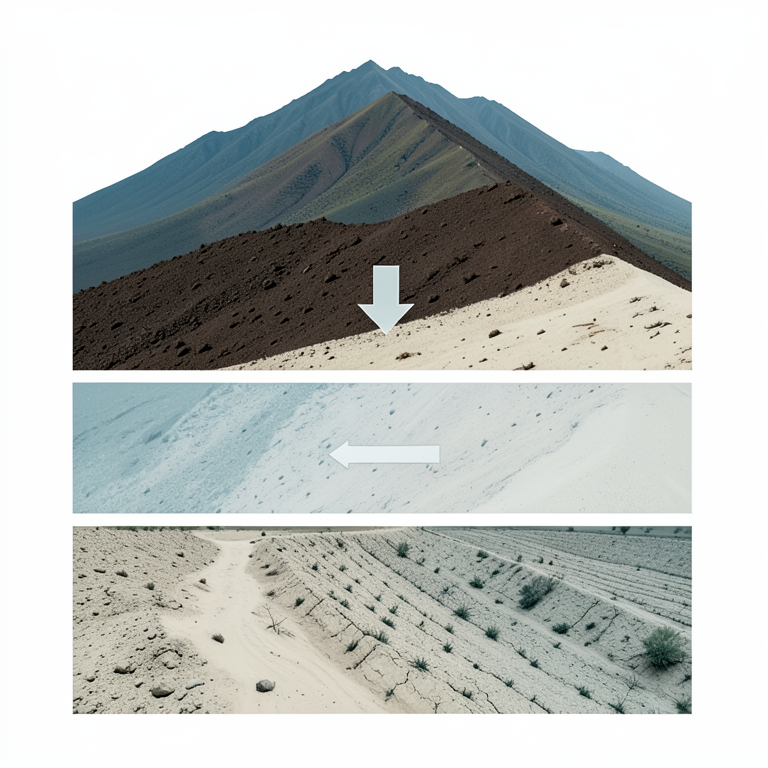
Elevation and Soil Quality Gradient
AI-generated conceptual illustration (Kenyan highland soil profiles across a mountain slope). It explains the idea and does not show study data.
View source evidence ↗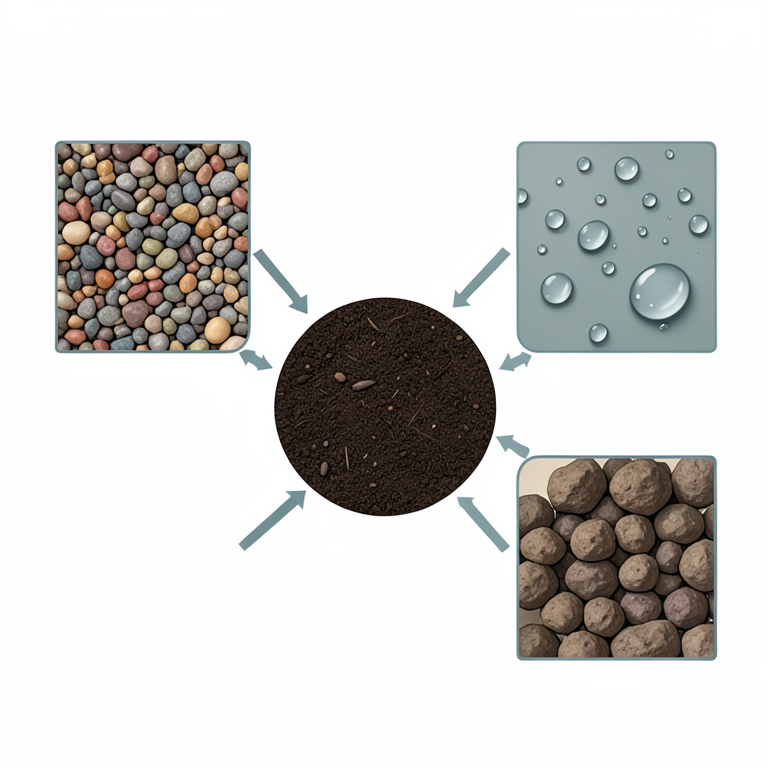
The Central Role of Organic Carbon
AI-generated conceptual illustration (Kenyan highland soil profiles with organic matter). It explains the idea and does not show study data.
View source evidence ↗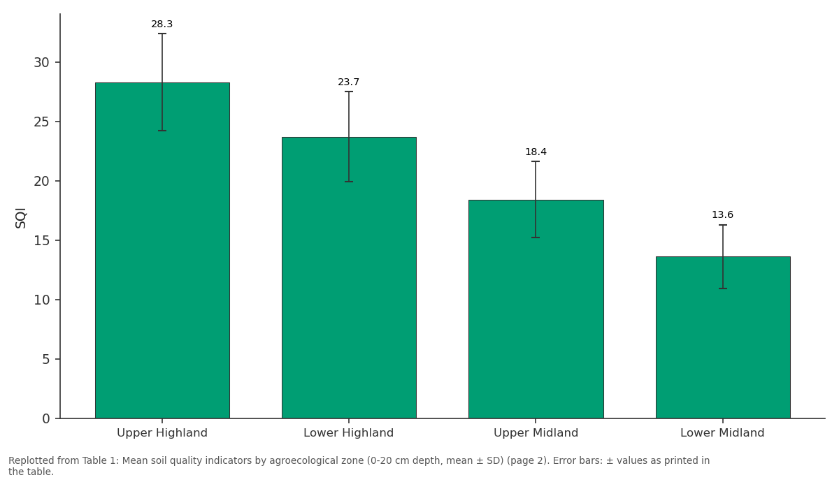
CEC: Upper Highland vs Lower Highland vs Upper Midland vs Lower Midland
Replotted from Table 1 (page 2) of the original paper. Every bar is the paper's own table value.
View source evidence ↗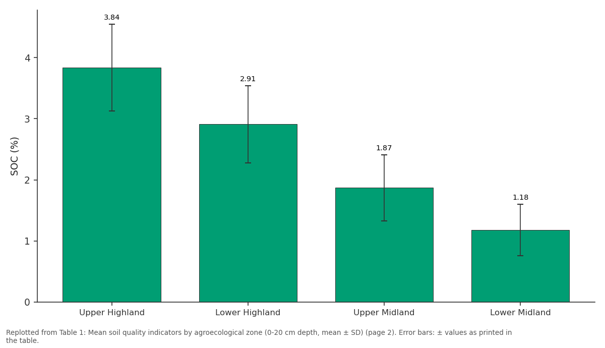
SOC (%): Upper Highland vs Lower Highland vs Upper Midland vs Lower Midland
Replotted from Table 1 (page 2) of the original paper. Every bar is the paper's own table value.
View source evidence ↗Figures & tables
From the original paper Table 1
 Table 2
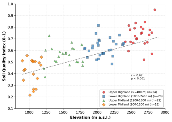 Figure 1
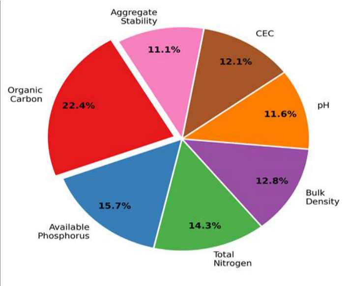 Figure 2
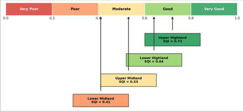 Figure 3
Introduction
The challenge is stark: Kenya's population is growing at 2.3% per year, arable land per capita has fallen below 0.12 hectares, and soil degradation affects an estimated 30% of cultivated area in the central highlands [1] . Soil quality-defined as the capacity of soil to function within ecosystem boundaries to sustain plant productivity, maintain environmental quality, and support human health [2] -is declining in many tropical highland systems under the combined pressures of intensive cropping, reduced fallow periods, and inadequate nutrient replenishment [3] . The Kenyan Highlands, stretching across Nyandarua, Nyeri, Meru, and Embu counties, produce the bulk of the country's maize, tea, coffee, and dairy output. They span an elevation range from roughly 900 m to over 3,000 m, encompassing several distinct agroecological zones (AEZs) that differ in rainfall, temperature, and dominant farming systems [4] . These AEZs create a natural gradient along which soil-forming factorsclimate, vegetation, and land use history-vary systematically, offering an opportunity to assess how soil quality responds to combined environmental and management pressures. Soil quality indices (SQIs) aggregate multiple soil properties into a single score that can be compared across sites and used to track change over time [5] . The most widely adopted approach follows three steps: indicator selection, scoring, and integration [6] . Principal component analysis (PCA) is often used to weight indicators objectively, and non-linear scoring functions accommodate the biological reality that crop response to soil properties is typically sigmoidal rather than linear [7] . Earlier applications of SQI methods in East Africa include Obade and Lal [8] in western Kenya and Vasu et al. [9] in the Ethiopian Highlands, but neither covered the full elevation range of the central Kenyan Highlands or tested the individual indicator perturbation. This research pursued three objectives: (a) to characterise soil physical, chemical, and biological properties across four AEZs in the central Kenyan Highlands, (b) to construct a PCA-weighted composite SQI and map its spatial variation along the elevation gradient, and (c) to evaluate, through sensitivity analysis, which soil indicators exert the strongest control on the composite index. The results are intended to inform county-level soil conservation planning by identifying both the zones most in need of intervention and the soil properties most worth targeting.
Materials and Methods
Materials and Methods
Materials
The research was conducted between April 2020 and September 2023 at Darwin College of Environmental Studies, Northern Territory, Australia, with four field campaigns in the central Kenyan Highlands (July 2020, March 2021, August 2022, February 2023). Ethical clearance was not required as no human subjects were involved. Research permits were obtained from the Kenya National Commission for Science, Technology and Innovation (NACOSTI permit P/21/10442, dated 8 April 2020). A total of 92 sampling sites were distributed across four AEZs: upper highland (>2,400 m, n = 24), lower highland (1,800-2,400 m, n = 28), upper midland (1,200-1,800 m, n = 22), and lower midland (900-1,200 m, n = 18). At each site, composite samples from five sub-samples within a 20 × 20 m plot were collected at 0-20 cm and 20-40 cm depths using a stainless-steel auger. Samples were airdried, sieved to < 2 mm, and shipped to the Darwin analytical laboratory.
Methods
Seven indicators were measured: soil organic carbon (SOC, Walkley-Black), total nitrogen (TN, Kjeldahl), available phosphorus (Olsen P), soil pH (1:2.5 H₂O), cation exchange capacity (CEC, ammonium acetate), bulk density (core method), and aggregate stability (wet-sieving mean weight diameter). Each indicator was scored on a 0-1 scale using non-linear scoring functions (sigmoidal or parabolic) calibrated against published crop-response thresholds for tropical highland soils [10] . PCA was run on the correlation matrix of the seven indicators; loadings from the first three components (explaining 68.3% of variance) were used to assign weights. The composite SQI was the weighted sum of normalised scores. Elevation-SQI relationships were tested with Pearson correlation and linear regression. Between-zone differences were assessed by one-way ANOVA with Tukey's HSD post-hoc test at p < 0.05.
Soil Quality Index Model and Parameterisation
The SQI model followed the additive weighted index framework of Andrews et al. [6] . For each indicator i, the raw measurement was transformed to a score Si ranging from 0 (worst observed) to 1 (optimal) using one of three scoring curves: 'more is better' (sigmoidal ascending) for SOC, TN, CEC, and aggregate stability; 'less is better' (sigmoidal descending) for bulk density; and 'optimum range' (bell-shaped) for pH and available P. Curve inflection points were set at the 10th and 90th percentiles of the dataset, and the midpoint was anchored to the published agronomic optimum for tropical Nitisols and Ferralsols [10,11] . The weight Wi for each indicator was the ratio of its absolute PCA loading on the dominant component to the sum of all loadings on that component. The composite SQI was computed as: SQI = Σ(Wi × Si), where the sum of all Wi equals 1. This approach ensures that indicators explaining the most variance in the dataset receive the highest influence on the final index, while the non-linear scoring captures threshold effects that linear normalisation would miss.
Sensitivity Analysis
A one-at-a-time perturbation analysis was performed to identify which indicators exert the strongest leverage on the composite SQI. Each indicator was varied by ±10% and ±20% around its measured value while all others were held constant, and the resulting change in SQI (ΔSQI) was recorded. The analysis was repeated for every sample (n = 92), and the mean absolute ΔSQI was reported per indicator. Organic carbon produced the largest mean ΔSQI (0.09 at ±20%), followed by available phosphorus (0.06) and total nitrogen (0.05). Bulk density and pH showed the smallest effects (both 0.03 at ±20%), consistent with their lower PCA loadings and the buffering effect of the bell-shaped scoring function for pH. The results confirm that management interventions targeting organic carbon inputs-cover cropping, composting, reduced tillage-would yield the greatest improvement in the composite soil quality score. All seven indicators declined from the upper highland to the lower midland zone. SOC dropped from 3.84% to 1.18%, and the composite SQI fell from 0.72 to 0.41. All pairwise zone comparisons were significant at p < 0.05 (Tukey's HSD, different letters in SQI column). The pie chart in Figure 2 confirms that organic carbon dominates the SQI (22.4%), consistent with its role as a master soil property influencing nutrient supply, water retention, and structural stability.
Results
Results
Comprehensive Interpretation
The data reveal a clear, elevation-linked gradient in soil quality across the Kenyan Highlands. Cooler temperatures, higher rainfall, and shorter cropping histories in the upper highland zone support higher organic matter accumulation and slower mineralisation, maintaining soil function. In the lower midland zone, warmer temperatures accelerate decomposition, longer cultivation histories have depleted nutrient reserves, and lower rainfall reduces biomass return to the soil.
Discussion
The SQI gradient from 0.72 in the upper highland to 0.41 in the lower midland is consistent with patterns reported by Obade and Lal [8] for western Kenya, who found SQI values of 0.68 on high-elevation tea soils and 0.38 on degraded sugarcane fields at lower elevations. The central highlands data extend this pattern by covering a wider elevation range and using a larger indicator set. The strong correlation between elevation and SQI (r = 0.67) reflects the combined influence of temperature on organic matter decomposition rates, rainfall on biomass production, and cultivation history on nutrient depletion-all of which co-vary with altitude in the Kenyan highlands [12,13] . That organic carbon carries the highest PCA weight (22.4%) and shows the greatest sensitivity (ΔSQI = 0.09 at ±20% perturbation) is consistent with its well-documented role as a master soil property. Organic carbon influences aggregate stability through binding agents, CEC through humic colloids, water holding capacity through hydrophilic functional groups, and nutrient supply through mineralisation [14] . Interventions that raise SOC-such as composting, cover cropping, mulching, and reduced tillage-would therefore have cascading positive effects on other soil properties and lift the composite SQI more efficiently than single-nutrient amendments [15,16] . The lower midland zone, where mean SQI falls below 0.50, is the most obvious priority for conservation investment. Soils here are subject to the highest cultivation intensity (two to three crops per year), the lowest residue return rates, and the warmest temperatures, creating a triple pressure on organic matter stocks [17] . Without targeted intervention, the trend toward further degradation appears likely to continue. A limitation of this research is the cross-sectional design, which captures spatial variation but cannot confirm temporal trends. Repeated sampling at the same sites over five to ten years would reveal whether SQI is declining, stable, or recovering under current management practices [18] . The SQI model itself depends on the choice of scoring functions and PCA-derived weights, both of which are sensitive to the dataset used; applying the same model to a different region may require recalibration [19] . Additionally, the 0-20 cm sampling depth captures the zone of greatest management influence but may underestimate subsoil constraints such as compaction or acidity below 40 cm [20] .
Conclusion
This research demonstrated a clear, elevation-linked gradient in soil quality across four agroecological zones of the central Kenyan Highlands. The composite soil quality index declined from 0.72 in the upper highland zone to 0.41 in the lower midland zone, with all seven indicators showing consistent downward trends along the gradient. Organic carbon was confirmed as the most influential indicator, carrying the highest PCA-derived weight (22.4%) and producing the largest response in sensitivity analysis. Lower midland soils, where the SQI fell below the 0.50 degradation threshold, represent the most pressing target for conservation investment. Management practices that raise organic carbon inputs-cover cropping, composting, reduced tillage, and agroforestry-would yield the greatest return on the composite index and should be prioritised in county soil management plans. The PCA-weighted SQI approach proved effective for integrating multiple soil properties into a single, spatially comparable metric. Its sensitivity to organic carbon aligns with agronomic experience and supports the case for carbon-centric soil health programmes across the East African highlands. Repeated sampling over time and extension of the framework to subsoil layers would strengthen its value as a monitoring tool for tracking progress toward sustainable land management targets [21] .
Acknowledgement
Acknowledgements Funding SourcesThis research was supported by departmental funds from Darwin College of Environmental Studies. No external grants are associated with this work. Institutional SupportThe authors acknowledge Darwin College for analytical laboratory access. NACOSTI is thanked for research clearance in Kenya.
Figures and tables from the paper
| AEZ | SOC (%) | TN (%) | P (ppm) | pH | BD | CEC | SQI |
|---|---|---|---|---|---|---|---|
| Upper Highland | 3.84±0.71 | 0.34±0.06 | 18.7±4.3 | 5.8±0.3 | 1.04±0.08 | 28.3±4.1 | 0.72±0.08a |
| Lower Highland | 2.91±0.63 | 0.27±0.05 | 14.2±3.8 | 5.6±0.4 | 1.12±0.09 | 23.7±3.8 | 0.64±0.09b |
| Upper Midland | 1.87±0.54 | 0.19±0.04 | 9.8±3.1 | 5.3±0.4 | 1.23±0.11 | 18.4±3.2 | 0.53±0.10c |
| Lower Midland | 1.18±0.42 | 0.13±0.03 | 6.4±2.4 | 5.1±0.5 | 1.34±0.12 | 13.6±2.7 | 0.41±0.11d |
Table text extracted from the original PDF; superscript letters are shown inline. The original table image is below.
View original table image
| Indicator | PC1 | PC2 | PC3 | Weight | Scoring Curve |
|---|---|---|---|---|---|
| Organic Carbon | 0.89 | 0.12 | 0.08 | 0.224 | More is better |
| Available P | 0.41 | 0.74 | 0.11 | 0.157 | Optimum range |
| Total Nitrogen | 0.82 | 0.18 | 0.14 | 0.143 | More is better |
| Bulk Density | −0.71 | 0.21 | −0.16 | 0.128 | Less is better |
Table text extracted from the original PDF; superscript letters are shown inline. The original table image is below.
View original table image
References
21 in the original paper- Jaetzold R, Schmidt H, Hornetz B, Shisanya C. Farm Management Handbook of Kenya, Vol. II. Ministry of Agriculture, Nairobi. 2006.
- Karlen DL, Mausbach MJ, Doran JW, Cline RG, Harris RF, Schuman GE. Soil quality: a concept, definition, and framework for evaluation. Soil Science Society of America Journal. 1997;61(1):4-10.
- Lal R. Restoring soil quality to mitigate soil degradation. Sustainability. 2015;7(5):5875-5895.
- Sombroek WG, Braun HMH, van der Pouw BJA. Exploratory soil map and agro-climatic zone map of Kenya. Kenya Soil Survey, Nairobi. 1982.
- Doran JW, Parkin TB. Defining and assessing soil quality. SSSA Special Publication. 1994;35:1-21.
- Andrews SS, Karlen DL, Cambardella CA. The soil management assessment framework. Soil Science Society of America Journal. 2004;68(6):1945-1962.
- Wymore AW. Model-Based Systems Engineering. CRC Press, Boca Raton. 1993.
- Obade VP, Lal R. Assessing land cover and soil quality by remote sensing and soil sampling. Geoderma. 2013;211-212:127-137.
- Vasu D, Singh SK, Ray SK, Duraisami VP, Tiwary P, Chandran P. Soil quality index for evaluation of degraded soils. Catena. 2016;141:32-40.
- Sanchez PA, Palm CA, Buol SW. Fertility capability soil classification. Geoderma. 2003;114(3-4):157-185.
- Shepherd KD, Walsh MG. Infrared spectroscopyenabling an evidence-based diagnostic surveillance approach to agricultural and environmental management in developing countries. Journal of Near Infrared Spectroscopy. 2007;15(1):1-19.
- Gicheru P, Gachene C, Mbuvi J, Mare E. Effects of soil management practices and tillage systems on surface soil water conservation and crust formation on a tropical Alfisol. American Journal of Alternative Agriculture. 2004;19(4):176-185.
- Batjes NH. Total carbon and nitrogen in the soils of the world. European Journal of Soil Science. 1996;47(2):151-163.
- Six J, Conant RT, Paul EA, Paustian K. Stabilization mechanisms of soil organic matter. Ecosystems. 2002;5(7):672-687.
- Lal R. Soil carbon sequestration impacts on global climate change and food security. Science. 2004;304(5677):1623-1627.
- Palm CA, Gachengo CN, Delve RJ, Cadisch G, Giller KE. Organic inputs for soil fertility management in tropical agroecosystems. Agriculture, Ecosystems and Environment. 2001;83(1-2):27-42.
- Tittonell P, Vanlauwe B, Leffelaar PA, Rowe EC, Giller KE. Exploring diversity in soil fertility management of smallholder farms in western Kenya. Agriculture, Ecosystems and Environment. 2005;110(34):166-184.
- Nandwa SM, Bekunda MA. Research on soil fertility in sub-Saharan Africa. Natural Resources Forum. 1998;22(4):231-243.
- Mairura FS, Mugendi DN, Mwanje JI, Ramisch JJ, Mbugua PK, Chianu JN. Integrating scientific and farmers' evaluation of soil quality indicators. Geoderma. 2007;139(1-2):134-143.
- Okalebo JR, Gathua KW, Woomer PL. Laboratory Methods of Soil and Plant Analysis. 2nd ed. TSBFCIAT, Nairobi. 2002.
- Kibblewhite MG, Ritz K, Swift MJ. Soil health in agricultural systems. Philosophical Transactions of the Royal Society B. 2008;363(1492):685-701.