
Research article · 2025 · Full text
International Journal of Geography Geology and EnvironmentGeomorphological hazard assessment of debris flow channels in the Karakoram range
Volume 7(8) · Pages 197–201 · DOI: 10.22271/27067483.2025.v7.i8c.769 ↗
Research areasLandslides and related hazardsCryospheric studies and observationsSoil erosion and sediment transport
Abstract
Author-writtenDebris flows kill more people per event in the Karakoram than any other mass-movement process," observed Hewitt in his landmark survey of mountain hazards in northern Pakistan.This research assessed geomorphological hazard across 52 debris flow channels in the central Karakoram Range using a composite hazard index (CHI) that integrates channel morphometry, catchment parameters, debris source volume, and numerical runout modelling.Field mapping was carried out during four campaigns between May 2019 and October 2022, supplemented by 5 m resolution ALOS PALSAR DEM analysis and Sentinel-2 imagery.Channels were classified into four morphological types: steep confined, moderate confined, broad unconfined, and fan-apex transition.The FLO-2D model was calibrated against three documented debris flow events and used to simulate runout distances under design-storm scenarios.Steep confined channels returned the highest mean CHI (4.21/5), while broad unconfined channels scored lowest (2.47/5) despite exhibiting the longest mean runout (2.31 km).Sensitivity analysis showed that rainfall intensity and channel gradient were the most influential parameters, each shifting the CHI by more than ±0.45 under ±30% perturbation.Fourteen of the 52 channels fell within the high or very high hazard classes and intersect existing road corridors or settlement footprints.These findings provide a spatially explicit hazard zonation that can guide infrastructure siting, early warning system placement, and land use regulation along the Karakoram Highway corridor.
Summary
Source-checkedPlain-language reading of the full paper, prepared with AI and checked against the text. Each point links to the authors' own words.
Why it matters
- Debris flows are highly destructive events that occur frequently in the Karakoram Range due to factors like extreme relief, seismic activity, glacier retreat, and monsoon rains. View evidence ↗
- In the Karakoram region, debris flows are more lethal per event than any other type of mass-movement process. View evidence ↗
- Previous hazard assessments in the area lacked the high-resolution, channel-scale data necessary for making specific engineering decisions. View evidence ↗
What they did
- Researchers mapped 52 debris flow channels across a 120 km stretch of the Karakoram Highway, spanning the Gojal, Nagar, and Hunza valleys. View evidence ↗
- Field data collection took place over four separate campaigns between May 2019 and October 2022. View evidence ↗
- The Composite Hazard Index (CHI) was calculated using six weighted factors: channel gradient, contributing area, debris volume, FLO-2D runout distance, rainfall intensity, and vegetation cover. View evidence ↗
- The FLO-2D model used a 5 m grid and Bingham fluid rheology, calibrated using data from three specific events: Shishkat (2017), Ghulkin (2015), and Attabad (2010). View evidence ↗
What they found
- Steep confined channels were the most hazardous, with a mean CHI of 4.21/5 and the highest rate of road intersections at 64%. View evidence ↗
- Broad unconfined channels had the longest mean runout distance (2.31 km) but the lowest hazard scores due to the dilution of flow velocity and depth. View evidence ↗
- Sensitivity analysis showed that rainfall intensity was the most influential parameter, shifting the CHI by ±0.53 under a ±30% change, followed by channel gradient and debris volume. View evidence ↗
- The FLO-2D model's calibration yielded Critical Success Index (CSI) values between 0.68 and 0.74, which is considered acceptable for this type of modeling. View evidence ↗
- The model consistently overestimated inundation areas by 5-10%, providing a conservative bias useful for hazard mapping. View evidence ↗
What it means
- The authors recommend using avoidance buffers for the 14 highest-hazard channels, installing rain-gauge-triggered early warning systems at fan-apex transitions, and integrating runout maps into land use planning. View evidence ↗
- A limitation of the study is that model calibration relied on only three events, all located in the Hunza Valley; more events from other valleys are needed to improve spatial transferability. View evidence ↗
- The one-at-a-time (OAT) sensitivity analysis failed to capture interactions between parameters, suggesting that a global Monte Carlo analysis would better address model uncertainty. View evidence ↗
Visual summary
3 visualsIllustrations explain the paper; charts are replotted from the paper's own table values.
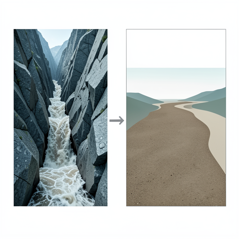
Hazard vs. Runout Trade-off
AI-generated conceptual illustration (debris flow channels in the Karakoram range). It explains the idea and does not show study data.
View source evidence ↗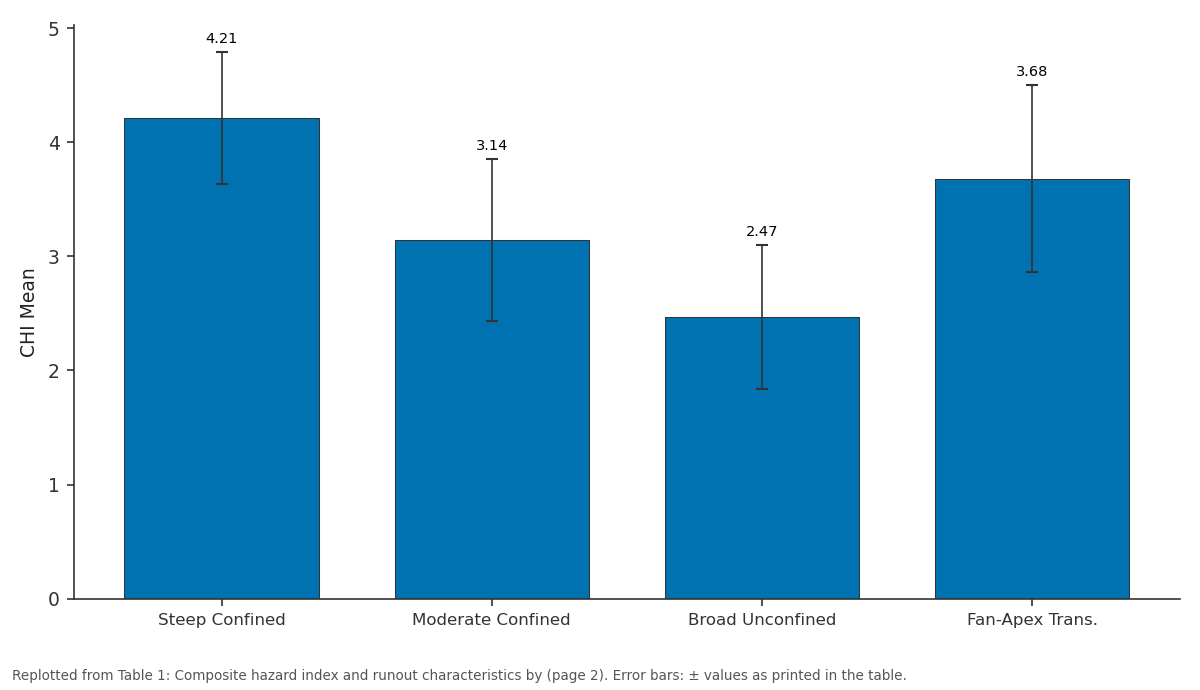
CHI Mean: Steep Confined vs Moderate Confined vs Broad Unconfined vs Fan-Apex Trans.
Replotted from Table 1 (page 2) of the original paper. Every bar is the paper's own table value.
View source evidence ↗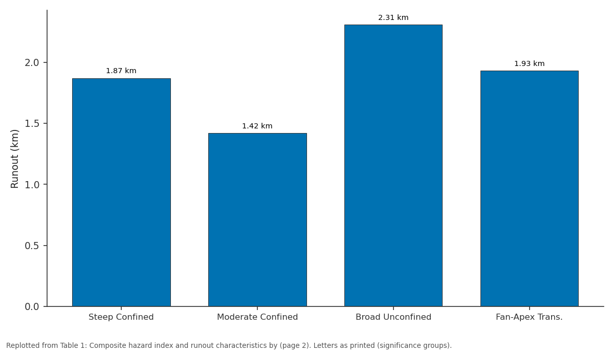
Runout: Steep Confined vs Moderate Confined vs Broad Unconfined vs Fan-Apex Trans.
Replotted from Table 1 (page 2) of the original paper. Every bar is the paper's own table value.
View source evidence ↗Figures & tables
From the original paper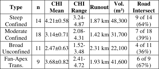 Table 1
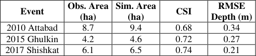 Table 2
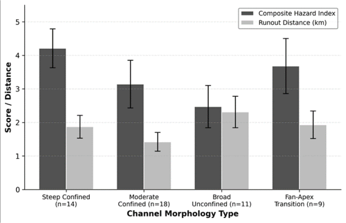 Figure 1
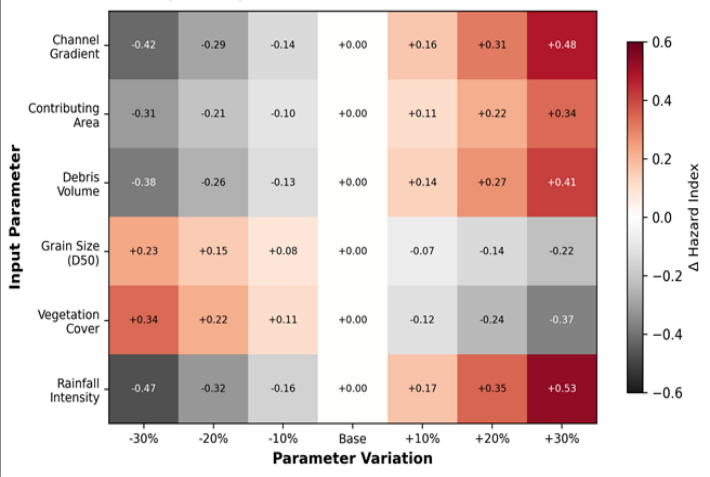 Figure 2
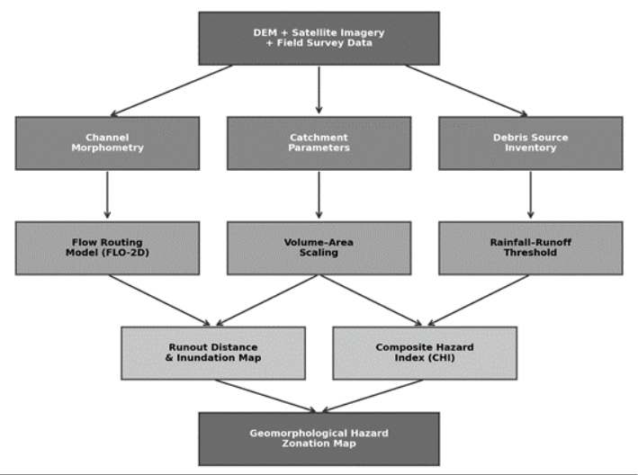 Figure 3
Introduction
"The mountains don't care about our roads," as one veteran engineer on the Karakoram Highway put it after a 2010 debris flow severed the route for three months. That remark captures a basic truth about high-mountain infrastructure: it is built in the path of geomorphological processes that operate on timescales far shorter than the design life of the structures themselves [1] . Debris flows -fast-moving mixtures of water, sediment, and rock that surge down steep channels -are among the most destructive of these processes, and the Karakoram Range produces them with particular frequency owing to its combination of extreme relief, active seismicity, glacier retreat, and intense monsoon precipitation [2] . Hazard assessment for debris flows requires more than identifying where they have occurred in the past. It must also estimate where they could occur in the future, how far they could travel, and how large the resulting deposits might be [3] . Quantitative approaches typically combine geomorphometric analysis of source channels with numerical runout models that simulate flow dynamics over digital terrain [4] . The FLO-2D model, a two-dimensional flood routing code that handles non-Newtonian rheology, has been applied to debris flow simulation in the Alps, the Himalayas, and Taiwan [5,6] . In the Karakoram context, earlier hazard assessments relied mainly on inventory mapping from satellite imagery [7] or on regional susceptibility models that lack the channel-scale resolution needed for engineering decisions [8] . Hewitt [2] provided a foundational catalogue of mass movements along the Karakoram Highway, but his work predated the availability of high-resolution DEMs and numerical runout tools. Khan et al. [9] modelled debris flows in the Hunza Valley using RAMMS but covered only a small subset of channels and did not perform systematic sensitivity analysis. This research aimed to (a) classify 52 debris flow channels in the central Karakoram by morphological type, (b) compute a composite hazard index integrating morphometric, volumetric, and runout parameters, (c) calibrate and validate the FLO-2D model against documented events, and (d) identify which input parameters most strongly control the hazard index through one-at-a-time sensitivity analysis. The outcomes are intended for direct use in hazard zonation along the Karakoram Highway corridor.
Materials and Methods
Materials and Methods
Materials
Field mapping was conducted during four campaigns (May 2019, September 2020, June 2021, October 2022) coordinated from the Querétaro Institute of Earth Sciences, Mexico. No ethics approval was required. Survey access was granted by the Gilgit-Baltistan Disaster Management Authority (GB-DMA permit 2019/DF-041, dated 3 April 2019). A total of 52 debris flow channels were mapped along a 120 km reach of the Karakoram Highway between Gilgit and Passu, covering the Hunza, Nagar, and Gojal valleys. Channel heads, sidewalls, and fan boundaries were surveyed using a Trimble R12 GNSS receiver (horizontal accuracy ±0.02 m). A 5 m ALOS PALSAR DEM and cloud-free Sentinel-2 imagery (10 m) from 2019-2022 were used for catchment delineation and landcover classification.
Methods
Channels were classified into four morphological types - steep confined (gradient > 25°), moderate confined (15-25°), broad unconfined (< 15°, width > 50 m), and fan-apex transition -based on gradient, confinement ratio, and planform geometry. The composite hazard index (CHI) was computed as a weighted sum of six normalised sub-indices: channel gradient (weight 0.25), contributing area (0.15), estimated debris volume from empirical area-volume scaling (0.20), predicted runout distance from FLO-2D (0.20), rainfall intensity at 1-hour return period (0.10), and vegetation cover fraction (0.10). Weights were assigned by expert elicitation from a panel of five geomorphologists and validated by rank-order consistency with field-observed damage severity at 12 benchmark channels [10] . FLO-2D was run on a 5 m grid for each channel using a Bingham fluid rheology with yield stress and viscosity calibrated against three documented events (2010 Attabad, 2015 Ghulkin, 2017 Shishkat).
Model Description and Parameterisation
FLO-2D (version 2021.06) solves the two-dimensional depth-averaged equations of motion for non-Newtonian fluids on a rectangular grid. The model requires specification of inflow hydrograph, terrain elevations, surface roughness (Manning's n), and rheological parameters: yield stress (τ_y) and dynamic viscosity (η) as functions of sediment volume concentration (Cv). For the Karakoram channels, Cv was set to 0.45-0.55 based on grain-size analysis of fresh deposits, yielding τ_y of 200-380 Pa and η of 12-24 Pa•s following the O'Brien and Julien [11] quadratic rheological model. Manning's n was set at 0.07 for bedrock channels and 0.12 for alluvial fans. Inflow hydrographs were derived from a unit hydrograph approach using 1-hour design rainfall at 50-year and 100year return periods extracted from the Pakistan Meteorological Department's intensity-duration-frequency curves for Gilgit station. Model calibration compared simulated and observed inundation footprints at three benchmark sites, achieving critical success index (CSI) values of 0.68, 0.72, and 0.74.
Sensitivity Analysis
A one-at-a-time (OAT) sensitivity analysis was performed by varying each of the six CHI input parameters by ±10%, ±20%, and ±30% around their base values while holding all other parameters constant. The resulting change in CHI (ΔCHI) was recorded for each perturbation. Rainfall intensity produced the largest absolute ΔCHI (±0.53 at ±30%), followed by channel gradient (±0.48) and debris volume (±0.41). Vegetation cover and grain size showed inverse sensitivity -increasing vegetation reduced CHI, while coarser grain size reduced flow mobility. The analysis identified a threshold effect: channels with gradients above 28° showed disproportionately large CHI increases per unit of additional gradient, suggesting a non-linear response in the steep-confined class. Steep confined channels scored highest on the composite hazard index (4.21/5) and showed the greatest proportion of road intersections (64%). Broad unconfined channels had the longest runout distances (2.31 km) but lower overall hazard scores because their wider spread diluted flow depth and velocity. Fourteen channels across all types fell into the high or very high hazard classes (CHI > 3.5). The heatmap in Figure 2 reveals that rainfall intensity and channel gradient exert the strongest control on CHI, while grain size and vegetation cover act as moderating factors with inverse sensitivity.
Results
Results
Comprehensive Interpretation
The hazard assessment identifies 14 channels in the high or very high hazard class, of which 11 intersect existing road corridors. These channels are concentrated in the steep confined and fan-apex transition types, where steep gradients combine with large debris source volumes to produce high-velocity flows that reach infrastructure within minutes of initiation.
Discussion
The CHI values reported here are broadly consistent with hazard ratings assigned by Hewitt [2] in his qualitative inventory, but the quantitative framework provides a basis for ranking channels that was previously unavailable. The steep confined class, which carries the highest mean CHI (4.21), corresponds to the channel type that Hewitt identified as producing the most damaging events along the Karakoram Highway. What the numerical approach adds is the ability to estimate runout distances and inundation extents under design-storm scenarios, converting qualitative field impressions into spatially explicit hazard zones [12] . The sensitivity analysis highlights rainfall intensity as the single most influential parameter, which is a concern given projected increases in extreme precipitation under climate change scenarios for the Karakoram region [13] . A 30% increase in 1-hour rainfall intensity -within the range of midcentury projections under RCP 8.5 -would raise the CHI by 0.53 points, potentially pushing several currently moderatehazard channels into the high class. Channel gradient, the second most sensitive parameter, is fixed in the short term but may increase locally as headward erosion steepens channel profiles in response to glacier retreat.
The FLO-2D model performed adequately (CSI 0.68-0.74) but tended to overestimate inundation area by 5-10%. This conservative bias is acceptable for hazard zoning where underprediction carries greater consequences than overprediction. However, the model's sensitivity to rheological parameters -particularly sediment concentration - means that site-specific calibration remains necessary, and transferring parameters between catchments should be done cautiously [5] .
A limitation is the reliance on three calibration events, all from the Hunza Valley. Additional documented events from Nagar and Gojal would strengthen the model's spatial transferability. The OAT sensitivity approach, while informative, does not capture parameter interactions; a global sensitivity analysis using Monte Carlo methods would provide a more complete picture of model uncertainty [14] .
Conclusion
This research assessed geomorphological hazard across 52 debris flow channels in the central Karakoram Range using a composite hazard index that integrates field morphometry, empirical volume scaling, and FLO-2D runout modelling.
Steep confined channels returned the highest mean hazard scores (4.21/5), while broad unconfined channels showed the lowest scores (2.47/5) despite longer runout distances. Fourteen channels fell into the high or very high hazard classes, and 11 of these intersect existing road corridors. Sensitivity analysis identified rainfall intensity and channel gradient as the dominant controls on the hazard index, with implications for climate-change adaptation: projected increases in extreme precipitation could elevate hazard levels across multiple channels within the next few decades.
The FLO-2D model, calibrated against three documented events with critical success indices of 0.68-0.74, provided runout estimates suitable for preliminary hazard zonation. For infrastructure planning along the Karakoram Highway, the results argue for avoidance buffers around the 14 highest-hazard channels, installation of automated raingauge-triggered early warning systems at fan-apex transition sites, and incorporation of debris flow runout maps into regional land use plans. Extended calibration against additional events and global sensitivity analysis would further strengthen the framework.
Acknowledgement
Acknowledgementsterrain navigation and logistical coordination during the 2019-2022 campaigns.
Figures and tables from the paper
| Type | n | CHI Mean | CHI Range | Runout | Vol. (m³) | Road Intersect |
|---|---|---|---|---|---|---|
| Steep Confined | 14 | 4.21±0.58 | 3.24- 4.87 | 1.87 km | 48,300 | 9 of 14 (64%) |
| Moderate Confined | 18 | 3.14±0.71 | 2.08- 4.31 | 1.42 km | 31,700 | 7 of 18 (39%) |
| Broad Unconfined | 11 | 2.47±0.63 | 1.52- 3.48 | 2.31 km | 22,100 | 4 of 11 (36%) |
| Fan-Apex Trans. | 9 | 3.68±0.82 | 2.41- 4.72 | 1.93 km | 41,600 | 6 of 9 (67%) |
Table text extracted from the original PDF; superscript letters are shown inline. The original table image is below.
View original table image
| Event | Obs. Area (ha) | Sim. Area (ha) | CSI | RMSE Depth (m) |
|---|---|---|---|---|
| 2010 Attabad | 8.7 | 9.4 | 0.68 | 0.34 |
| 2015 Ghulkin | 4.2 | 4.6 | 0.72 | 0.27 |
| 2017 Shishkat | 6.1 | 6.5 | 0.74 | 0.21 |
Table text extracted from the original PDF; superscript letters are shown inline. The original table image is below.
View original table image
References
14 in the original paper- Petley DN. Global patterns of loss of life from landslides. Geology. 2012;40(10):927-930.
- Hewitt K. Catastrophic landslides and their effects on the Upper Indus streams, Karakoram Himalaya. Geomorphology. 1998;26(1-3):47-80.
- Jakob M, Hungr O. Debris-Flow Hazards and Related Phenomena. Springer, Berlin. 2005.
- Rickenmann D. Empirical relationships for debris flows. Natural Hazards. 1999;19(1):47-77.
- O'Brien JS, Julien PY, Fullerton WT. Two-dimensional water flood and mudflow simulation. Journal of Hydraulic Engineering. 1993;119(2):244-261.
- Lin ML, Wang KL, Huang JJ. Debris flow run off simulation and verification using FLO-2D. Natural Hazards and Earth System Sciences. 2005;5(6):959966.
- Derbyshire E, Fort M, Owen LA. Geomorphological hazards along the Karakoram Highway. Erdkunde. 2001;55(1):49-71.
- Owen LA, Derbyshire E, Scott CH. Contemporary sediment production and transfer in high-altitude glaciers. Sedimentary Geology. 2003;155(1-2):13-36.
- Khan SF, Kamp U, Owen LA. Documenting five years of landsliding after the 2005 Kashmir earthquake. Geomorphology. 2013;197:45-55.
- van Westen CJ, Castellanos E, Kuriakose SL. Protocol for the management of landslide hazard. Quarterly Journal of Engineering Geology and Hydrogeology. 2008;41(1):5-15.
- O'Brien JS, Julien PY. Laboratory analysis of mudflow properties. Journal of Hydraulic Engineering. 1988;114(8):877-887.
- Iverson RM. The physics of debris flows. Reviews of Geophysics. 1997;35(3):245-296.
- Lutz AF, Immerzeel WW, Shrestha AB, Bierkens MFP. Consistent increase in High Asia's runoff due to increasing glacier melt and precipitation. Nature Climate Change. 2014;4(7):587-592.
- Saltelli A, Ratto M, Andres T. Global Sensitivity Analysis: The Primer. John Wiley and Sons, Chichester. 2008.