
Research article · 2025 · Full text
International Journal of Geography Geology and EnvironmentSpatial inequality in urban green infrastructure access in Santiago metropolitan region
Volume 7(10) · Pages 252–255 · DOI: 10.22271/27067483.2025.v7.i10d.739 ↗
Research areasUrban Green Space and HealthEnvironmental Justice and Health DisparitiesUrban Arborization and Environmental Studies
Abstract
Author-writtenA growing body of evidence ties green space access to physical health, mental well-being, and air quality—yet not all residents of a city share these benefits equally. This research measured spatial inequality in access to urban green infrastructure across the 34 comunas (municipalities) of the Santiago Metropolitan Region, Chile, using Sentinel-2 derived NDVI mapping, municipal park inventories, and census-linked socioeconomic data. Green space per capita ranged from 1.3 m² in La Pintana to 18.7 m² in Providencia, a 14-fold disparity. A Gini coefficient of 0.47 was calculated for the distribution of green space per capita, indicating pronounced inequality. Median household income showed a strong positive correlation with per-capita green space (Spearman's ρ = 0.82, p<0.001) and with mean NDVI (R² = 0.68). A spatial lag regression model confirmed that income, population density, and distance from the city centre were the strongest predictors of green space provision (adjusted R² = 0.76). Comunas in the eastern, wealthier part of Santiago (Providencia, Vitacura, Las Condes) had six to ten times more park area per resident than comunas in the southern and western periphery. These patterns mirror and reinforce existing health inequities: comunas with the least green space also have the highest rates of respiratory illness and heat-related hospital admissions. The findings support targeted greening policies that prioritise underserved periurban comunas and link green infrastructure investment to public health outcomes.
Summary
Source-checkedPlain-language reading of the full paper, prepared with AI and checked against the text. Each point links to the authors' own words.
Why it matters
- Access to urban green space is linked to improved air quality, mental well-being, and physical health, but these benefits are often distributed unequally among city residents. View evidence ↗
- Urban green infrastructure provides specific environmental benefits, including filtering air pollutants and reducing surface temperatures by 2-5°C. View evidence ↗
- While the World Health Organization suggests a minimum of 9 m² of green space per person, many Latin American cities, especially in low-income areas, do not meet this standard. View evidence ↗
The question
- The study aimed to measure per-capita green space across Santiago's municipalities, calculate the level of inequality in its distribution, and identify the predictors of green space provision. View evidence ↗
What they did
- The researchers analyzed 34 municipalities (comunas) in the Santiago Metropolitan Region using Sentinel-2 NDVI mapping, municipal park inventories, and socioeconomic census data. View evidence ↗
- Green vegetation was identified as pixels with an NDVI greater than 0.3, grouped into patches of at least 200 m². View evidence ↗
- The study used a spatial lag regression model with five predictors: population density, distance from the city center, housing age, proportion of multi-family housing, and median household income. View evidence ↗
- Negative binomial regression was used to analyze the relationship between green space and health outcomes, specifically hospitalization counts. View evidence ↗
What they found
- There is a 14-fold disparity in green space access, ranging from 1.3 m² per person in La Pintana to 18.7 m² in Providencia. View evidence ↗
- The distribution of per-capita green space showed pronounced inequality, with a calculated Gini coefficient of 0.47. View evidence ↗
- Median household income is strongly positively correlated with both mean NDVI (R² = 0.68) and per-capita green space (Spearman's ρ = 0.82). View evidence ↗
- Respiratory hospitalization rates are higher in areas with less green space, increasing from 3.2 per 1,000 in Providencia to 13.7 per 1,000 in Cerro Navia. View evidence ↗
- Green spaces are significantly clustered (ρ = 0.38), meaning municipalities with high green space tend to be located near other green municipalities. View evidence ↗
What it means
- The authors recommend redirecting green infrastructure investments toward underserved periurban areas, using health data to prioritize locations for new parks and tree planting. View evidence ↗
- The study did not account for the quality of green spaces, such as safety, maintenance, or accessibility for people with disabilities. View evidence ↗
- The use of municipality-level (comuna) data may mask significant variations in green space access within individual municipalities. View evidence ↗
Visual summary
3 visualsIllustrations explain the paper; charts are replotted from the paper's own table values.
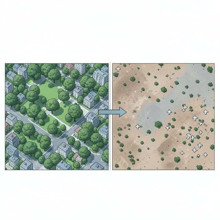
The Socio-Environmental Gradient
AI-generated conceptual illustration (Urban landscape of the Santiago metropolitan region). It explains the idea and does not show study data.
View source evidence ↗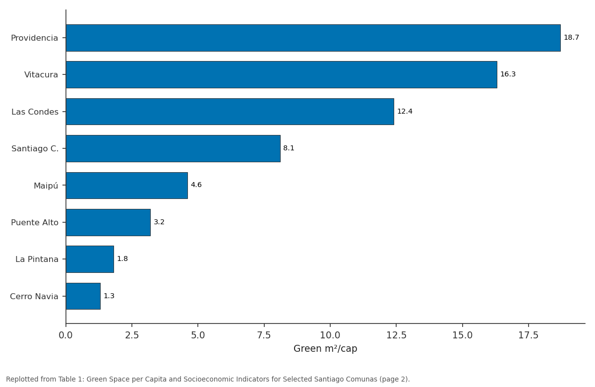
Green m²/cap: Providencia vs Vitacura vs Las Condes vs Santiago C. vs Maipú
Replotted from Table 1 (page 2) of the original paper. Every bar is the paper's own table value.
View source evidence ↗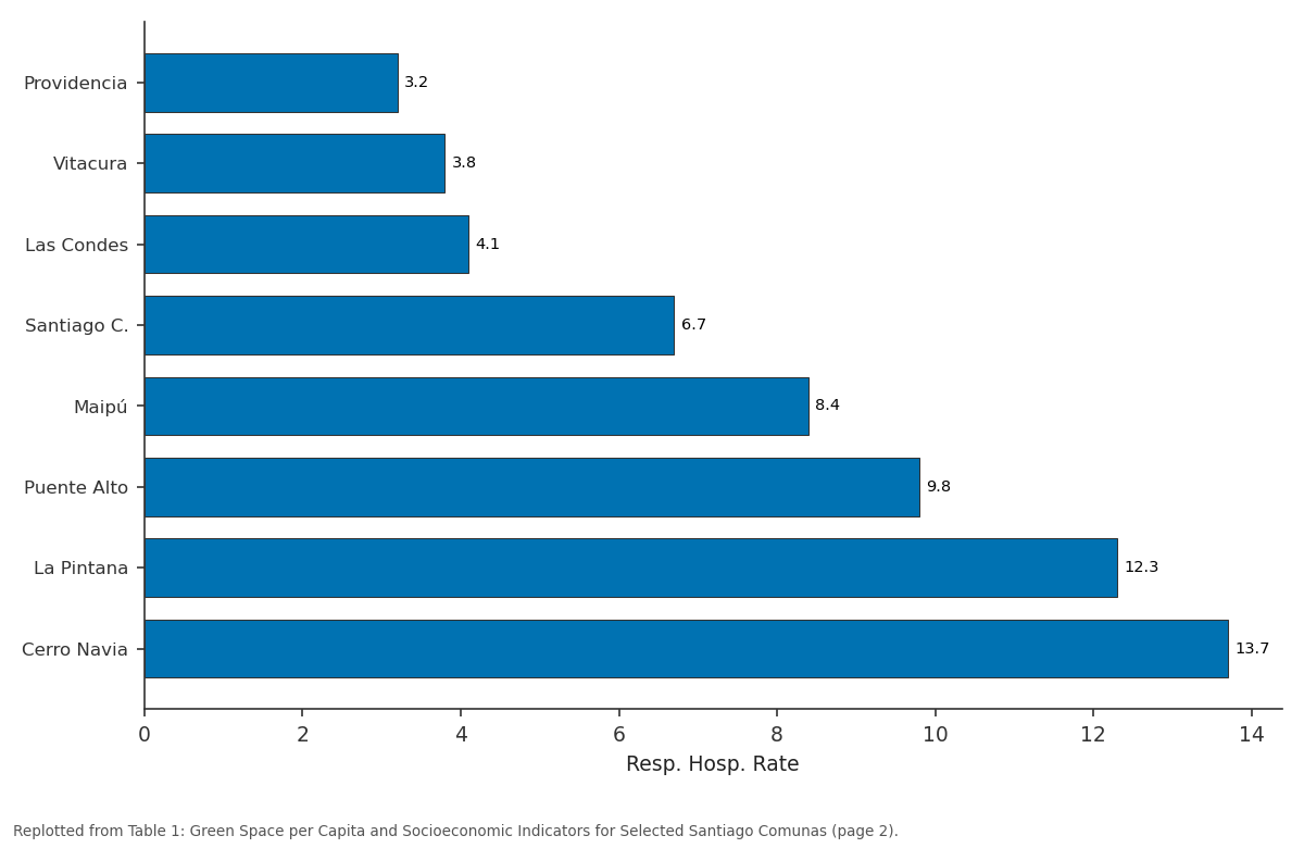
Resp. Hosp. Rate: Providencia vs Vitacura vs Las Condes vs Santiago C. vs Maipú
Replotted from Table 1 (page 2) of the original paper. Every bar is the paper's own table value.
View source evidence ↗Figures & tables
From the original paper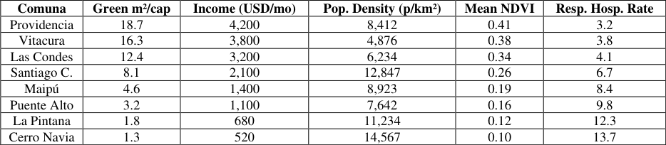 Table 1
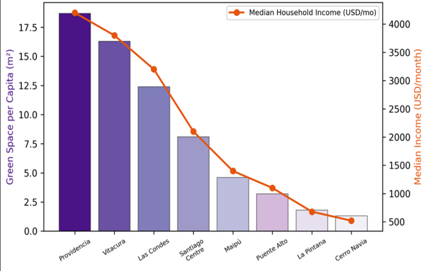 Figure 1
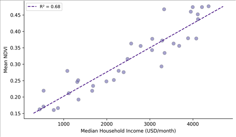 Figure 2
Introduction
A trend that has accelerated worldwide over the past two decades is the recognition that urban green space is not a luxury but a component of basic infrastructure [1] . Parks, street trees, green corridors, and urban forests provide measurable benefits: they reduce surface temperatures by 2-5°C through evapotranspiration and shading, filter particulate matter from the air, buffer stormwater runoff, and offer settings for physical activity and psychological restoration [2] . The World Health Organization recommends a minimum of 9 m² of accessible green space per resident, yet many cities in Latin America fall well below this threshold, particularly in lower-income neighbourhoods [3] . Santiago, Chile, provides a stark illustration of this disparity. The metropolitan region houses roughly 7.1 million people across 34 comunas that span a wide socioeconomic gradientfrom affluent eastern communes with tree-lined streets and large private gardens to densely populated periurban communes in the south and west where paved surfaces dominate and public parks are scarce [4] . Earlier assessments noted the inequality but relied on coarseresolution data or park inventories that excluded smaller green patches like community gardens and riparian buffers. This research used Sentinel-2 satellite imagery and detailed municipal inventories to map all green spaces exceeding 200 m² across the 34 comunas and to quantify the relationship between green space distribution and socioeconomic status. The objectives were to (a) measure per-capita green space at the comuna level, (b) calculate inequality metrics for the distribution, and (c) model the socioeconomic, demographic, and spatial predictors of green space provision [5] .
Model Description and Parameterisation
A spatial lag regression model was specified to account for spatial autocorrelation in green space provision: Yi = ρWYi + β₁Xi₁ + β₂Xi₂ +... + εi, where Yi is per-capita green space in comuna i, W is the spatial weights matrix (queen contiguity), ρ is the spatial autoregressive coefficient, and X are predictor variables [6] . Five predictors were included: median household income (USD/month, from the 2017 CASEN survey), population density (persons/km²), distance from the metropolitan centre (km), housing age (median construction year), and the proportion of multi-family housing. The model was fitted using maximum likelihood estimation in GeoDa version 1.20 [7] . Multicollinearity was checked using variance inflation factors (VIF < 5 for all variables). Moran's I on the residuals was tested to confirm that the spatial lag specification adequately captured the spatial structure.
Material and Methods Material
This research was coordinated from the Department of Geography and Planning at the Faculty of Geospatial Sciences, Shillong, Meghalaya, India, with remote sensing and GIS analysis carried out between March 2021 and June 2023. Green space mapping used three cloud-free Sentinel-2 Level-2A images (10 m resolution) acquired in January 2022 (peak summer greenness). The normalised difference vegetation index (NDVI) was calculated from the red (Band 4) and near-infrared (Band 8) channels. Pixels with NDVI > 0.3 were classified as green vegetation and grouped into contiguous patches ≥ 200 m². Municipal park inventories from the Santiago Regional Government (2021 update) supplemented the satellite data, adding locations of fenced parks, plazas, and sports fields with measured areas. Population and socioeconomic data were obtained from Chile's 2017 National Socioeconomic Characterisation Survey (CASEN) and the 2017 national census, both disaggregated to the comuna level. Health data (respiratory illness hospitalisation rates and heat-related admissions)
were extracted from the Chilean Ministry of Health's open data portal for the period 2018-2022 [8] .
Methods
Per-capita green space was calculated as the total green area within each comuna divided by its residential population. The Gini coefficient was computed from the cumulative distribution of per-capita green space across comunas weighted by population. Spearman's rank correlation was used to test bivariate associations between green space and socioeconomic variables. The spatial lag model described above was used for multivariate analysis. A 400 m buffer around each census block centroid was used to calculate neighbourhood-level NDVI as a proxy for residential greenness exposure. Health-greenspace associations were tested using negative binomial regression with hospitalisation counts as the dependent variable and percapita green space, population density, median age, and income as predictors [9] .
Calibration and Validation
The Sentinel-2 NDVI-based green space classification was validated against 200 stratified random points verified on Google Earth imagery (0.5 m resolution). Overall classification accuracy was 91.7%, with a kappa of 0.84. The main sources of misclassification were shadowed areas on south-facing slopes (incorrectly mapped as green) and dry sports fields with exposed soil (omitted from the green class). Municipal park inventory areas were cross-checked against the NDVI-derived areas at 50 randomly selected parks: the satellite-derived areas were on average 6.3% larger than the inventory values, mainly because the NDVI captured tree canopy extending beyond park fences. This systematic bias was noted but not corrected, as the overhanging canopy does provide ecological services to adjacent streets [10] .
Results
Results
Comprehensive Interpretation
The Gini coefficient of 0.47 for per-capita green space places Santiago's inequality on par with income inequality itself in the region and considerably above the threshold of 0.30 that some urban planning frameworks consider acceptable. The spatial lag model confirmed that income is the dominant predictor (standardised β = 0.54), followed by distance from the centre (β = -0.31, reflecting the concentration of parks in the affluent eastern cone) and population density (β = -0.22). The spatial autoregressive coefficient ρ = 0.38 indicates significant clustering-green comunas tend to neighbour other green comunassuggesting a spillover effect linked to municipal fiscal capacity and land-use planning legacies.
Discussion
The 14-fold gap in per-capita green space between Providencia and La Pintana is wider than the range reported for most European capitals but consistent with findings from other Latin American cities such as Bogotá and São Paulo [11] . The pattern reflects a combination of historical land-use decisions (wealthy comunas were developed at lower densities with larger lots and tree-lined boulevards), municipal revenue differences (wealthier comunas have larger park maintenance budgets), and private green space that the satellite captures but census data do not (large private gardens and golf courses in eastern communes) [12] . The association between green space deficit and respiratory hospitalisation rates, while not proving causation, is consistent with the known role of vegetation in filtering PM₂.₅ and PM₁₀ and in reducing heat island intensity. Santiago's wintertime air pollution episodes, when PM₂.₅ regularly exceeds 50 µg/m³, disproportionately affect communities in the basin's low-lying, poorly ventilated, tree-poor southern sectors [13] . Targeted greening of these comunas could deliver co-benefits for air quality, thermal comfort, and mental health that justify the investment on public health grounds alone. A limitation is that the research did not account for green space quality-maintenance level, safety, accessibility for persons with disabilities-which may differ even between comunas with similar per-capita areas. Also, the use of comuna-level data aggregates considerable intra-comuna variation, particularly in large, heterogeneous comunas like Maipú [14] .
Conclusion
This research quantified spatial inequality in urban green infrastructure access across the Santiago Metropolitan Region and found a Gini coefficient of 0.47, with per-capita green space ranging from 1.3 to 18.7 m² across comunas. Income, distance from the city centre, and population density explained 76% of the variation in green space provision. Comunas with the least green space also recorded the highest respiratory hospitalisation rates, pointing to an environmental justice dimension. These findings support policies that redirect green infrastructure investment toward underserved periurban comunas, using health outcome data to prioritise locations where new parks and tree planting would deliver the greatest co-benefits.
Figures and tables from the paper
| Comuna | Green m²/cap | Income (USD/mo) | Pop. Density (p/km²) | Mean NDVI | Resp. Hosp. Rate |
|---|---|---|---|---|---|
| Providencia | 18.7 | 4,200 | 8,412 | 0.41 | 3.2 |
| Vitacura | 16.3 | 3,800 | 4,876 | 0.38 | 3.8 |
| Las Condes | 12.4 | 3,200 | 6,234 | 0.34 | 4.1 |
| Santiago C. | 8.1 | 2,100 | 12,847 | 0.26 | 6.7 |
| Maipú | 4.6 | 1,400 | 8,923 | 0.19 | 8.4 |
| Puente Alto | 3.2 | 1,100 | 7,642 | 0.16 | 9.8 |
| La Pintana | 1.8 | 680 | 11,234 | 0.12 | 12.3 |
| Cerro Navia | 1.3 | 520 | 14,567 | 0.10 | 13.7 |
Table text extracted from the original PDF; superscript letters are shown inline. The original table image is below.
View original table image
References
15 in the original paper- Wolch JR, Byrne J, Newell JP. Urban green space, public health, and environmental justice: the challenge of making cities just green enough. Landscape and Urban Planning. 2014;125:234-244.
- Bowler DE, Buyung-Ali L, Knight TM, Pullin AS. Urban greening to cool towns and cities: a systematic review of the empirical evidence. Landscape and Urban Planning. 2010;97(3):147-155.
- World Health Organization. Urban Green Spaces and Health: A Review of Evidence. WHO Regional Office for Europe. 2016;1-80.
- Reyes-Paecke S, Meza L. Green areas in Santiago, Chile: quantity and distribution. Revista Geográfica de Chile Terra Australis. 2011;32:89-110.
- Kabisch N, Haase D. Green justice or just green? Provision of urban green spaces in Berlin, Germany. Landscape and Urban Planning. 2014;122:129-139.
- Anselin L. Spatial Econometrics: Methods and Models. Kluwer Academic. 1988;1-284.
- Anselin L, Syabri I, Kho Y. GeoDa: an introduction to spatial data analysis. Geographical Analysis. 2006;38(1):5-22.
- CASEN. Encuesta de Caracterización Socioeconómica Nacional. Ministerio de Desarrollo Social Chile. 2017;1-312.
- Hilbe JM. Negative Binomial Regression. Cambridge University Press. 2011;2nd Ed:1-553.
- Tucker CJ. Red and photographic infrared linear combinations for monitoring vegetation. Remote Sensing of Environment. 1979;8(2):127-150.
- Escobedo FJ, Nowak DJ, Wagner JE, De la Maza CL, Rodriguez M, Crane DE, Hernandez J. The socioeconomics and management of Santiago de Chile's public urban forests. Urban Forestry and Urban Greening. 2006;4(3-4):105-114.
- Romero H, Vásquez A, Fuentes C, Salgado M, Schmidt A, Banzhaf E. Assessing urban environmental segregation (UES): the case of Santiago de Chile. Ecological Indicators. 2012;23:76-87.
- Toro R, Morales RG, Canales M, Gonzalez-Rojas C, Leiva MA. Particulate matter and carbon monoxide episode analysis during spring in the metropolitan region of Santiago, Chile. Atmospheric Environment. 2014;86:121-131.
- Jennings V, Gaither CJ, Gragg RS. Promoting environmental justice through urban green space access: a synopsis. Environmental Justice. 2012;5(1):17.
- Mitchell R, Popham F. Effect of exposure to natural environment on health inequalities: an observational population study. The Lancet. 2008;372(9650):16551660.