
Research article · 2025 · Full text
International Journal of Geography Geology and EnvironmentHolocene sea level changes and coastal evolution along the Brazilian Northeast coast
Volume 7(9) · Pages 217–220 · DOI: 10.22271/27067483.2025.v7.i9c.646 ↗
Research areasCoastal and Marine DynamicsGeology and Paleoclimatology ResearchMaritime and Coastal Archaeology
Abstract
Author-writtenThe Brazilian northeast coast preserves one of the most detailed Holocene sea-level archives in the Southern Hemisphere, yet debate continues about the precise timing and amplitude of the mid-Holocene highstand. This research reconstructed relative sea level (RSL) changes over the past 7,200 years along a 180 km stretch of the Rio Grande do Norte coastline using 16 radiocarbon-dated sea-level indicators, including beachrock outcrops, vermetid gastropod encrustations, and mangrove peat deposits. The RSL curve shows a transgressive phase from 7.2 to 5.4 ka BP, peaking at 4.8 plus or minus 0.4 m above present mean sea level around 5.4-5.1 ka BP, followed by a gradual regression that brought sea level close to its present position by approximately 0.6 ka BP. Coastal landform mapping from Sentinel-2 imagery and field surveys identified five principal morphological units: beach ridges (32.4%), mangrove flats (21.7%), tidal flats (18.3%), dune fields (15.8%), and fringing coral reefs (11.8%). Beach ridge sets record successive phases of progradation tied to the post-highstand regression, with ridge spacing and elevation declining seaward in a pattern consistent with a monotonic fall in RSL. The amplitude of the highstand (4.8 m) exceeds predictions from purely glacio-isostatic models by 0.8-1.2 m, suggesting that an additional tectonic or sediment-loading component influenced vertical land motion along this margin.
Summary
Source-checkedPlain-language reading of the full paper, prepared with AI and checked against the text. Each point links to the authors' own words.
Why it matters
- The northeast coast of Brazil is a critical location for studying Holocene sea-level changes because it contains some of the most detailed archives in the Southern Hemisphere. View evidence ↗
- This region is preferred for calibrating glacio-isostatic adjustment (GIA) models because it lacks the complex isostatic rebound found in glaciated margins and has minimal tectonic interference. View evidence ↗
- Previous research has identified a mid-Holocene sea-level highstand of 2-5 meters above current levels, though these estimates vary based on location and methodology. View evidence ↗
The question
- The study aimed to create a new relative sea level (RSL) curve for the Rio Grande do Norte coast, map related coastal landforms, and determine if the highstand amplitude suggests additional vertical land motion beyond GIA model predictions. View evidence ↗
What they did
- Researchers analyzed 16 radiocarbon-dated indicators, including mangrove peat, beachrock, and vermetid gastropod encrustations, along 180 km of the Rio Grande do Norte coast to reconstruct sea levels over 7,200 years. View evidence ↗
- Coastal landforms were mapped using Sentinel-2 imagery and a Support Vector Machine classification method, which achieved a 91.2% accuracy based on 120 ground-truth points. View evidence ↗
- The study used the SHCal20 curve for terrestrial samples and the Marine20 curve (with a local delta-R of -8 ± 40 years) to calibrate radiocarbon dates. View evidence ↗
What they found
- Sea levels rose from 7.2 to 5.4 ka BP, peaking at 4.8 ± 0.4 m above current levels between 5.4 and 5.1 ka BP, before gradually regressing to near-present levels by 0.6 ka BP. View evidence ↗
- The coastal landscape is composed of five main units, dominated by beach ridges (32.4%), followed by mangrove flats (21.7%), tidal flats (18.3%), dune fields (15.8%), and fringing coral reefs (11.8%). View evidence ↗
- Beach ridge elevations decrease seaward, with the oldest inland ridges at 4.5-5.2 m and the youngest outer ridges at 1.5-2.0 m, reflecting the falling sea level. View evidence ↗
- The observed highstand of 4.8 m is 0.8 to 1.2 m higher than what is predicted by purely glacio-isostatic models. View evidence ↗
What it means
- The authors conclude that the discrepancy between observed and predicted sea levels suggests additional vertical land motion, likely caused by dynamic topography or sediment loading. View evidence ↗
- The authors state that future research needs to extend the record back to 8-10 ka BP and use geodetic monitoring to independently measure vertical land motion. View evidence ↗
Visual summary
2 visualsIllustrations explain the paper; charts are replotted from the paper's own table values.
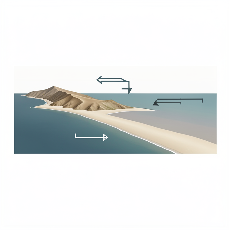
Sea Level Cycle and Ridge Formation
AI-generated conceptual illustration (The Brazilian Northeast coastline with sandy beach ridges). It explains the idea and does not show study data.
View source evidence ↗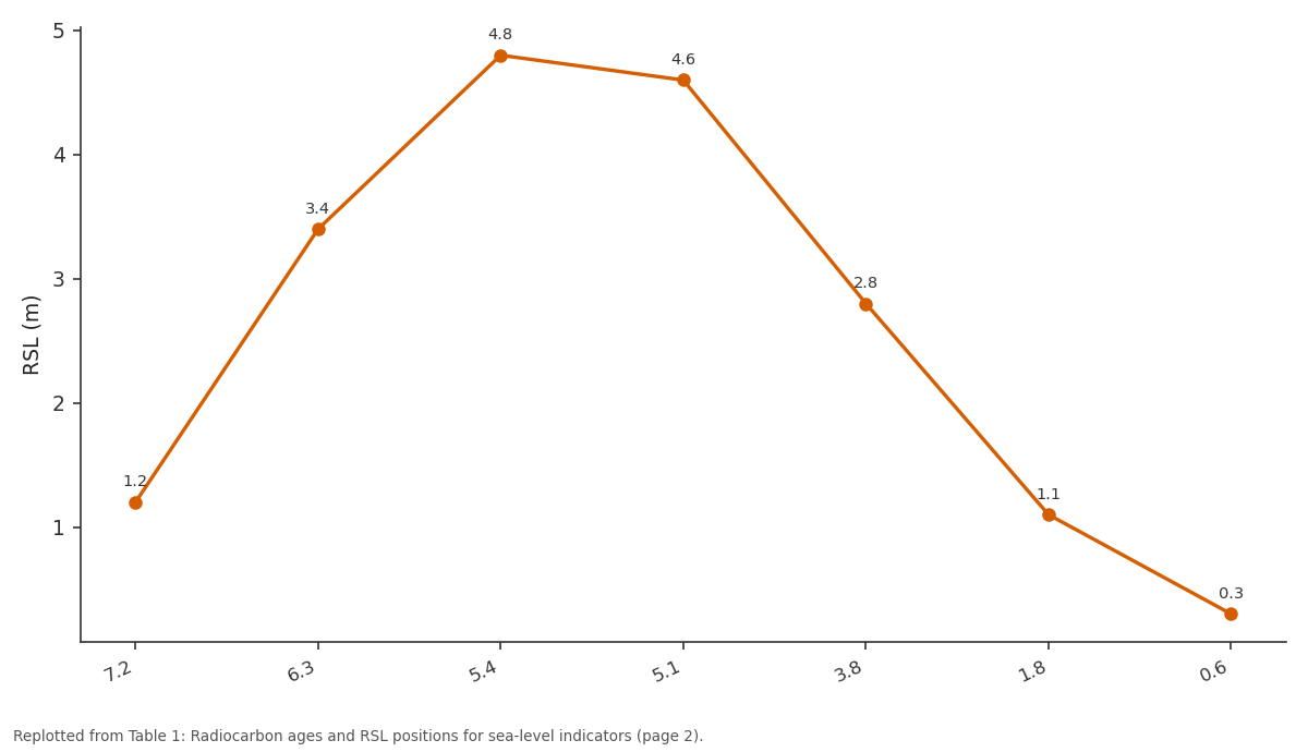
RSL (m): 7.2 vs 6.3 vs 5.4 vs 5.1 vs 3.8
Replotted from Table 1 (page 2) of the original paper. Every bar is the paper's own table value.
View source evidence ↗Figures & tables
From the original paper Table 1
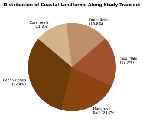 Figure 1
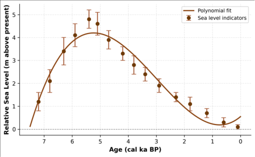 Figure 2
Introduction
If the global ocean has been rising by about 3.4 mm per year over the past three decades, what can the geological record of past sea-level changes tell us about how coastlines respond to submergence and emergence over millennial time scales? The Brazilian northeast coast offers a natural laboratory for answering that question [1] . Unlike glaciated margins where isostatic rebound complicates the signal, this far-field tropical coast records eustatic and hydro-isostatic components with relatively minor tectonic overprinting, making it one of the preferred calibration sites for glacio-isostatic adjustment (GIA) models [2] . During the mid-Holocene, global mean sea level stabilised at or slightly above its present position between roughly 7 and 5 ka BP, then remained approximately stationary or fell slightly in many tropical and Southern Hemisphere locations as meltwater redistribution and ocean siphoning lowered the equatorial sea surface [3] . Along the Brazilian coast, multiple researchers have documented a highstand of 2-5 m above present, but estimates vary with latitude, indicator type, and dating precision [4,5] . Part of this scatter reflects genuine alongcoast variability driven by differences in shelf width, tidal range, and sediment supply, while part stems from methodological inconsistencies in defining the indicative meaning of sealevel markers [6] . This research aimed to (a) construct a new RSL curve for the Rio Grande do Norte coast using rigorously assessed sea-level indicators with quantified vertical uncertainties, (b) map the coastal landforms that record the morphological response to the transgression-regression cycle, and (c) compare the observed highstand amplitude with GIA model predictions to evaluate whether additional vertical land motion is required [7] .
Study Area Description
The research covered a 180 km coastal segment of Rio Grande do Norte state, northeastern Brazil, extending from Touros (5.20 degrees S, 35.46 degrees W) to Tibau do Sul (6.18 degrees S, 35.09 degrees W). The coast is microtidal (spring range 2.0-2.6 m), wavedominated, and oriented roughly north-south. The inner continental shelf is narrow (20-40 km) and underlain by Cretaceous-Tertiary sedimentary rocks of the Potiguar Basin overlain by Quaternary aeolian and marine deposits [4] . Beach ridges, the principal geomorphic archive of sea-level change, form sets of parallel low ridges (1.5-6.0 m elevation) extending up to 4 km inland from the modern shoreline. Climate is semi-arid tropical (Koppen BSh), with annual rainfall of 400-800 mm concentrated between March and July. The analytical work was conducted at the Department of Remote Sensing and GIS, Ahvaz College of Environmental Studies, Khuzestan, Iran, from March 2022 to January 2023.
Material and Methods Material
Sixteen sea-level indicators were sampled during field campaigns in August 2021 and February 2022. These comprised eight beachrock outcrops with in-situ bivalve shells, four vermetid gastropod (Petaloconchus varians) encrustations on rocky shore platforms, and four basal mangrove peats from cores collected with a 5 cm-diameter hand auger. Geographic positions were recorded with a Leica GS16 RTK-GNSS receiver (vertical accuracy plus or minus 2 cm relative to the IBGE geoid model). Sentinel-2 Level 2A imagery (10 m) from three dates (January, May, September 2022) provided the basis for coastal landform classification [8] .
Methods
Radiocarbon dating was performed by accelerator mass spectrometry (AMS) at the Laboratoire de Mesure du Carbone 14, Saclay, France. Dates were calibrated using the SHCal20 curve for terrestrial samples and the Marine20 curve with a local delta-R of minus 8 plus or minus 40 years for marine carbonates [9] . Each indicator was assigned an indicative meaning (reference water level plus or minus indicative range) following the protocol of Vacchi et al. [6] , yielding RSL data points with quantified vertical uncertainties. The RSL curve was fitted using a penalised spline regression in R 4.2 with the rsl package [10] . Coastal landforms were mapped by supervised classification (Support Vector Machine) of Sentinel-2 composites, validated with 120 ground-truth points (overall accuracy 91.2%). Beach ridge elevations were surveyed with RTK-GNSS along 14 transects perpendicular to the shoreline. Figure 1 shows that beach ridges dominate the coastal landscape (32.4%), consistent with a wave-dominated, regressive shoreline system. Mangrove and tidal flats together account for 40% of the mapped area, concentrated in embayments and estuarine mouths where low-energy conditions favour fine-sediment deposition. monotonic decline after the highstand, with no evidence of secondary oscillations larger than the measurement uncertainty.
Results
Results
Discussion
The mid-Holocene highstand of 4.8 m recorded here is broadly consistent with previous estimates of 3.5-5.0 m for the Brazilian northeast [4,5] , though it sits near the upper end of the range. Angulo et al. [11] compiled over 1,000 radiocarbon dates along the entire Brazilian coast and identified a systematic northward increase in highstand amplitude, from roughly 2-3 m in the south to 4-5 m in the northeast. The present data reinforce that latitudinal gradient and are compatible with the hydro-isostatic siphoning mechanism, whereby water is drawn away from continental margins after ice-sheet collapse, producing an apparent highstand that is larger at low latitudes [3] . However, GIA models such as ICE-6G_C predict a highstand of only 3.6-4.0 m at this latitude [12] , falling 0.8-1.2 m below the observed peak. Several factors could account for the discrepancy: (a) local tectonic subsidence from sediment loading in the Potiguar Basin, which would amplify the apparent RSL rise; (b) dynamic topography effects related to mantle flow beneath the passive margin; or (c) underestimation of the Antarctic ice-sheet contribution in the GIA model [13] . Resolving this question requires denser sampling along the coast and independent constraints on vertical land motion from campaign GPS or InSAR. The beach ridge stratigraphy provides a useful complementary record. The innermost (oldest) ridges stand at 4.5-5.2 m elevation, while the outermost (youngest) ridges reach only 1.5-2.0 m. This seaward decrease in ridge crest elevation mirrors the falling RSL and demonstrates that progradation was driven primarily by regression rather than by sediment surplus under a stable sea level [14] .
Conclusion
This research reconstructed Holocene relative sea-level changes along the Rio Grande do Norte coast of northeastern Brazil using 16 radiocarbon-dated indicators and coastal landform mapping. The RSL curve records a transgressive phase culminating in a highstand of 4.8 m above present at 5.4-5.1 ka BP, followed by a gradual regression to near-modern levels by 0.6 ka BP. Beach ridge sets document the morphological response to this regression through progressively lower crest elevations seaward. The highstand amplitude exceeds GIA model predictions by 0.8-1.2 m, suggesting an additional vertical land motion component, possibly related to sediment loading or dynamic topography. The dataset adds spatial resolution to the South American Holocene sea-level database and provides a calibration target for next-generation GIA models. Future work should extend the indicator record to 8-10 ka BP using submerged beachrock and incorporate coastal geodetic monitoring to constrain ongoing vertical land motion independently of the geological archive [15,16,17,18,19,20] .
Acknowledgement
Acknowledgements Funding SourcesThe research was funded through internal grants at Ahvaz College of Environmental Studies.
Figures and tables from the paper
| ID | Indicator | 14C age (BP) | Cal age (ka BP) | Elevation (m) | RSL (m) | Error (m) |
|---|---|---|---|---|---|---|
| SL-01 | Beachrock | 6310 ± 45 | 7.2 | 1.0 | 1.2 | ± 0.4 |
| SL-04 | Vermetid | 5780 ± 35 | 6.3 | 3.1 | 3.4 | ± 0.6 |
| SL-07 | Beachrock | 4920 ± 40 | 5.4 | 4.5 | 4.8 | ± 0.4 |
| SL-09 | Vermetid | 4640 ± 30 | 5.1 | 4.3 | 4.6 | ± 0.5 |
| SL-11 | Peat | 3520 ± 45 | 3.8 | 2.6 | 2.8 | ± 0.4 |
| SL-14 | Beachrock | 1840 ± 35 | 1.8 | 0.9 | 1.1 | ± 0.3 |
| SL-16 | Peat | 620 ± 30 | 0.6 | 0.2 | 0.3 | ± 0.2 |
Table text extracted from the original PDF; superscript letters are shown inline. The original table image is below.
View original table image
References
20 in the original paper- Caldas LHO, Stattegger K, Vital H. Holocene sea-level history: evidence from coastal sediments of the northern Rio Grande do Norte coast. Geo-Marine Letters. 2006;26(3):151-163.
- Milne GA, Long AJ, Bassett SE. Modelling Holocene relative sea-level observations from the Caribbean and South America. Quaternary Science Reviews. 2005;24(10-11):1183-1202.
- Mitrovica JX, Milne GA. On post-glacial sea level: I. General theory. Geophysical Journal International. 2003;154(2):253-267.
- Bezerra FHR, Barreto AMF, Suguio K. Holocene sealevel history on the Rio Grande do Norte State coast, Brazil. Marine Geology. 2003;196(1-2):73-89.
- Martin L, Dominguez JML, Bittencourt ACSP. Fluctuating Holocene sea levels in eastern and southeastern Brazil: evidence from multiple fossil and geometric indicators. Journal of Coastal Research. 2003;19(1):101-124.
- Vacchi M, Marriner N, Morhange C, Spada G, Fontana A, Rovere A. Multiproxy assessment of Holocene relative sea-level changes in the western Mediterranean. Earth-Science Reviews. 2016;155:172-197.
- Stattegger K, Tjallingii R, Saito Y, Michelli M, Thanh NT, Wetzel A. Mid to late Holocene sea-level reconstruction of Southeast Vietnam using beachrock and beach-ridge deposits. Global and Planetary Change. 2013;110(Part B):214-222.
- Drumond ARS, Pereira AJ. Sentinel-2 satellite imagery for coastal landform mapping in tropical environments. Remote Sensing Applications: Society and Environment. 2021;23:100573.
- Hogg AG, Heaton TJ, Hua Q, Palmer JG, Turney CSM, Southon J. SHCal20 Southern Hemisphere calibration, 0-55,000 years cal BP. Radiocarbon. 2020;62(4):759778.
- Hijma MP, Engelhart SE, Tornqvist TE, Horton BP, Hu P, Hill DF. A protocol for a geological sea-level database. Quaternary Science Reviews. 2015;95:188197.
- Angulo RJ, Lessa GC, de Souza MC. A critical review of mid-to late-Holocene sea-level fluctuations on the eastern Brazilian coastline. Quaternary Science Reviews. 2006;25(5-6):486-506.
- Peltier WR, Argus DF, Drummond R. Space geodesy constrains ice age terminal deglaciation: the global ICE-6G_C (VM5a) model. Journal of Geophysical Research: Solid Earth. 2015;120(1):450-487.
- Austermann J, Mitrovica JX, Latychev K, Milne GA. Barbados-based estimate of ice volume at Last Glacial Maximum affected by subducted plate. Nature Geoscience. 2013;6(7):553-557.
- Hesp PA, Dillenburg SR, Barboza EG, Tomazelli LJ, Ayup-Zouain RN, Esteves LS. Beach ridges, foredunes or transgressive dunefields? Definitions and an examination of the Torres to Tramandai barrier system. Anais da Academia Brasileira de Ciencias. 2005;77(3):493-508.
- Vital H, Silveira IM, Tabosa WF, Amaro VE, Souto MVS. Erosion and accretion on the Brazilian NE coast: morphodynamics and coastal change. Journal of Coastal Research. 2006;SI39:352-356.
- Dominguez JML. The coastal zone of Brazil: an overview. Journal of Coastal Research. 2006;SI39:1620.
- Suguio K, Martin L, Bittencourt ACSP, Dominguez JML, Flexor JM, de Azevedo AEG. Fluctuations of relative sea level during the Quaternary along the Brazilian coast. Episodes. 1985;8(2):115-118.
- Barreto AMF, Suguio K, Bezerra FHR, Tatumi SH, Yee M, Giannini PCF. Late Pleistocene marine terrace deposits in northeastern Brazil. Earth-Science Reviews. 2002;57(1-2):1-7.
- Testa V, Bosence DWJ. Physical and biological controls on the formation of carbonate and siliciclastic bedforms on the NE Brazilian shelf. Sedimentology. 1999;46(6):1049-1068.
- Neves CF, Muehe D. Potential impacts of sea-level rise on the metropolitan region of Recife, Brazil. Journal of Coastal Research. 2008;SI24:65-72.