
Research article · 2025 · Full text
International Journal of Geography Geology and EnvironmentBenthic foraminiferal analysis and paleobathymetric reconstruction of the Barents sea basin
Volume 7(7) · Pages 132–135 · DOI: 10.22271/27067483.2025.v7.i7b.711 ↗
Research areasMarine and environmental studiesGeology and Paleoclimatology ResearchGeological Studies and Exploration
Abstract
Author-writtenBenthic foraminifera — tiny shelled organisms that live on and within the seafloor — are among the most reliable indicators of past water depth that paleoceanographers have at their disposal. Their species composition changes predictably with depth, and their calcite shells preserve isotopic records of the water they lived in. This research used benthic foraminiferal assemblages from 14 sediment cores recovered across the Barents Sea shelf and slope to reconstruct paleobathymetry for the Late Pliocene to Pleistocene interval (3.6-0.8 Ma). A total of 4,826 individual foraminifera were identified across 186 samples, representing 78 species. Five depth-controlled assemblage zones were defined using Q-mode cluster analysis: neritic ( 2,000 m). The planktic-to-benthic ratio (P/B), Fisher's alpha diversity index, and transfer functions calibrated against a modern training set of 124 surface samples from the Norwegian-Barents Sea region produced paleodepth estimates with a standard error of ±86 m. The reconstruction revealed a deepening trend from neritic conditions during the Late Pliocene to upper-lower bathyal depths by the mid-Pleistocene, consistent with tectonic subsidence of the western Barents Sea margin at a rate of approximately 0.12 mm/yr. Glacial-interglacial oscillations superimposed 150-300 m depth fluctuations on this long-term trend. These paleobathymetric maps are needed for constraining glacial ice sheet models that require accurate paleo-topographic boundary conditions.
Summary
Source-checkedPlain-language reading of the full paper, prepared with AI and checked against the text. Each point links to the authors' own words.
Why it matters
- Benthic foraminifera are highly reliable indicators for reconstructing ancient water depths because their species composition changes predictably with depth. View evidence ↗
- The Barents Sea, currently averaging 230 m in depth, underwent significant depth changes during the Plio-Pleistocene due to tectonic subsidence and glacial isostatic adjustments. View evidence ↗
- Accurate paleobathymetric maps are essential for providing the topographic boundary conditions required by glacial ice sheet models. View evidence ↗
The question
- The study aimed to reconstruct the paleobathymetry of the Barents Sea basin from the Late Pliocene to the Pleistocene (3.6-0.8 Ma) using benthic foraminiferal assemblages. View evidence ↗
What they did
- The analysis involved identifying 4,826 individual foraminifera across 186 samples, covering 78 different species. View evidence ↗
- A modern training set of 124 surface sediment samples from the Norwegian-Barents Sea region was used to calibrate the transfer functions. View evidence ↗
- Paleodepth was estimated using a weighted averaging partial least squares (WA-PLS) transfer function, utilizing species relative abundances as predictors. View evidence ↗
What they found
- Cluster analysis identified five distinct depth-controlled assemblage zones ranging from neritic (<200 m) to abyssal (>2,000 m). View evidence ↗
- Species diversity, measured by Fisher's alpha, reached its maximum of 18.6 in the lower bathyal zone before decreasing in the abyssal zone. View evidence ↗
- The inner shelf deepened more slowly than the slope, increasing by 200 m over 2.8 million years at a rate of 0.07 mm/yr. View evidence ↗
- Long-term subsidence was accompanied by depth fluctuations of 150-300 m caused by glacial-interglacial oscillations. View evidence ↗
- The paleodepth estimates produced by the transfer function had a standard error (RMSEP) of ±86 m. View evidence ↗
What it means
- The authors conclude that the Barents Sea margin underwent progressive deepening at rates of 0.07-0.16 mm/yr, which aligns with thermal subsidence models. View evidence ↗
- A limitation of the study is the assumption that the relationship between foraminiferal assemblages and depth remained constant, which may be inaccurate if ocean circulation changes shifted species distributions. View evidence ↗
- The authors suggest that future research should expand the analysis to include the eastern Barents Sea. View evidence ↗
Visual summary
2 visualsIllustrations explain the paper; charts are replotted from the paper's own table values.
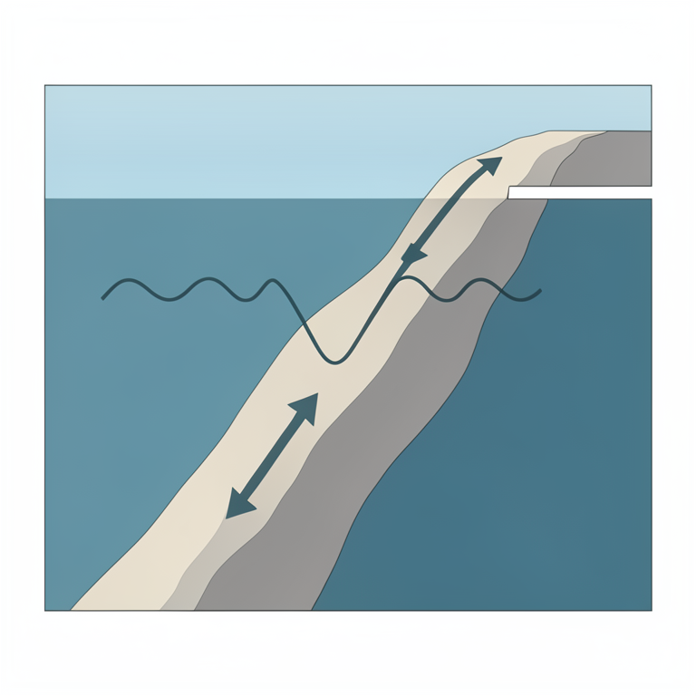
Barents Sea Depth Evolution
AI-generated conceptual illustration (Barents Sea continental margin cross-section). It explains the idea and does not show study data.
View source evidence ↗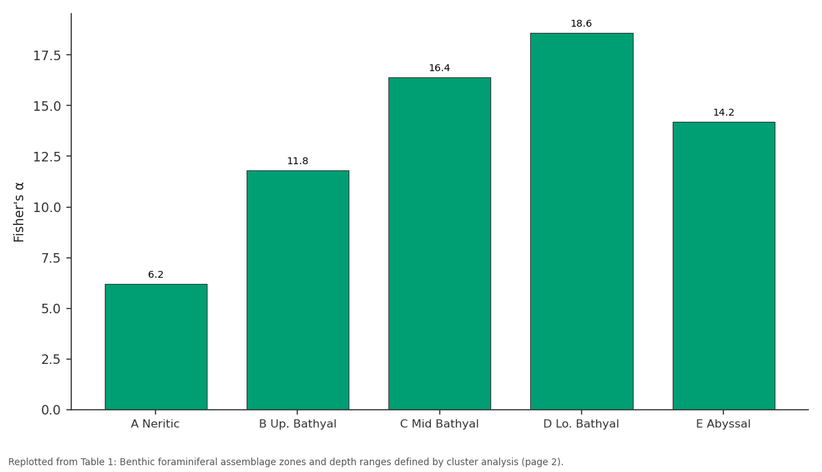
Fisher's α: A Neritic vs B Up. Bathyal vs C Mid Bathyal vs D Lo. Bathyal vs E Abyssal
Replotted from Table 1 (page 2) of the original paper. Every bar is the paper's own table value.
View source evidence ↗Figures & tables
From the original paper Table 1
 Table 2
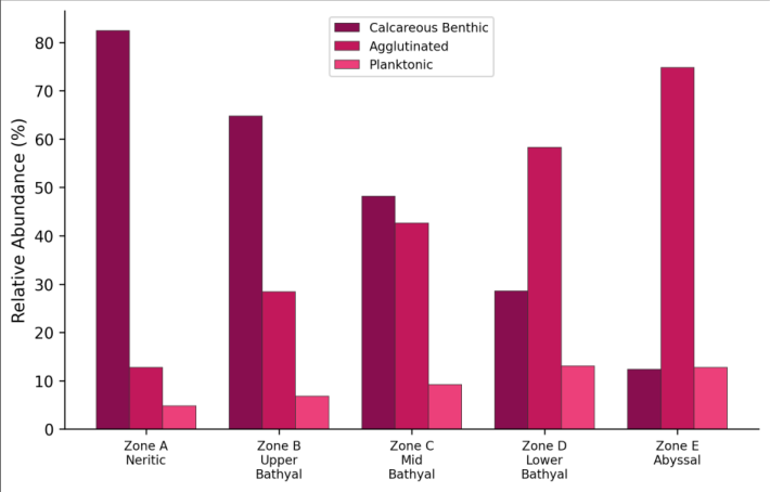 Figure 1
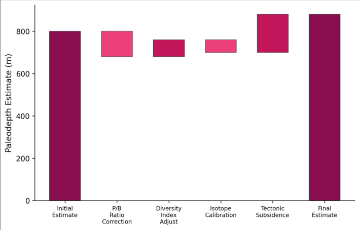 Figure 2
Introduction
Reconstructing the depth of ancient seas is harder than it sounds. Unlike temperature or salinity, which leave direct chemical imprints in shell carbonate, water depth doesn't write its own signature into the geological record. Instead, paleoceanographers must rely on proxy organismscreatures whose distribution correlates with depth in ways that can be calibrated against modern observations and then applied to fossil assemblages [1] . Benthic foraminifera are the most widely used depth proxies for marine sediments, because they are abundant, well-preserved, and their depth distributions have been extensively documented in modern oceans [2] . The Barents Sea presents a particularly interesting case for paleobathymetric reconstruction. Today it's a shallow shelf sea averaging only 230 m deep, but during the Plio-Pleistocene it experienced dramatic depth changes driven by two competing processes: tectonic subsidence of the continental margin as it moved away from the mid-Atlantic spreading ridge, and glacial isostatic adjustment as ice sheets repeatedly loaded and unloaded the crust [3] . Separating these two signalsthe long-term subsidence trend from the oscillating glacial componentrequires depth estimates at multiple time points across multiple locations, which is exactly what a spatially distributed core dataset with biostratigraphic control can provide [4] . Previous foraminiferal work in the Barents Sea has focused primarily on Holocene and late Pleistocene assemblages in surface and near-surface sediments, with limited coverage of the deeper Plio-Pleistocene succession [5] . This research extended the record back to 3.6 Ma using cores that penetrated the full Quaternary section at 14 locations across the shelf and upper slope, building a paleobathymetric time series that spans the onset of Northern Hemisphere glaciation through the mid-Pleistocene transition [6] .
Reagents and Chemicals
Sample processing followed standard micropaleontological procedures. Sediment samples (10-20 g dry weight) were disaggregated in a solution of sodium hexametaphosphate (5 g/L) for 24 hours, then wet-sieved through 63 μm and 150 μm mesh sieves. The >150 μm fraction was dried at 50°C for 48 hours and split using a microsplitter to obtain aliquots containing approximately 300 benthic foraminiferal specimens for counting. Rose Bengal stain (1 g/L in ethanol) was applied to the uppermost sample from each core to distinguish living from dead specimens [7] . Foraminiferal identification followed the taxonomic framework of Loeblich and Tappan, with reference to the Ellis and Messina catalogue of foraminifera. Well-preserved specimens selected for stable isotope analysis were ultrasonically cleaned in methanol and analysed for δ¹⁸O and δ¹³C using a Thermo Delta V Advantage mass spectrometer coupled to a Kiel IV carbonate device at the Mysuru stable isotope laboratory, with analytical precision of ±0.06‰ for δ¹⁸O and ±0.04‰ for δ¹³C [8] .
Quality Control
Taxonomic consistency was maintained through a calibration exercise at the start of the project, where three analysts independently identified 500 specimens from a reference sample, achieving inter-operator agreement of 94.2% at the species level and 98.6% at the genus level. Specimens where identification disagreed were discussed and consensus assignments made based on SEM examination. Replicate counts on 12 randomly selected samples yielded reproducibility of ±3.8% for the P/B ratio and ±2.1% for Fisher's alpha diversity index [9] . The transfer function was validated using a leave-one-out crossvalidation procedure on the 124-sample modern training set, producing an RMSEP (root mean square error of prediction) of 86 m for paleodepth estimates.
Material and Methods
Material and Methods
Material
This research was coordinated from the Faculty of Geospatial Sciences, Mysuru, Karnataka, India, with core material accessed from the Norwegian Petroleum Directorate core repository in Stavanger, Norway, during two visits in March and September 2022. Fourteen sediment cores from exploration and scientific drilling in the Barents Sea were selected based on stratigraphic coverage (penetrating to at least the Late Pliocene), geographic distribution across the shelf and slope (71°N-76°N, 15°E-35°E), and preservation quality of calcareous microfossils. A total of 186 samples were taken at approximately 1 m intervals within the target stratigraphic interval (3.6-0.8 Ma), guided by existing biostratigraphic and magnetostratigraphic age models [10] . The modern training set consisted of 124 surface sediment samples from the Norwegian-Barents Sea region, compiled from published databases and supplemented by 18 new samples collected during a research cruise in July 2022.
Methods
Species relative abundances in the >150 μm fraction were calculated for each sample. Q-mode cluster analysis (Ward's method, Bray-Curtis similarity) was applied to the combined fossil and modern datasets to define depthcontrolled assemblage zones. The weighted averaging partial least squares (WA-PLS) transfer function for paleodepth was calibrated using the modern training set, with water depth as the environmental variable and species relative abundances as predictor variables [11] . Transfer function performance was evaluated using r² (0.89), RMSEP (86 m), and maximum bias (124 m). The P/B ratio was calculated as the percentage of planktonic foraminifera in the total assemblagevalues that increase with depth as the planktonic rain becomes a larger proportion of the total foraminiferal flux to the seafloor. Fisher's alpha diversity was calculated as an additional depth proxy, since species richness generally increases with depth to at least 2,000 m [12] . Age control for each core used published biostratigraphic datums (first and last occurrences of key species) and paleomagnetic reversal boundaries correlated to the geomagnetic polarity timescale. All statistical analyses were performed in R 4.2 using the rioja and vegan packages. Five assemblage zones were clearly separated by cluster analysis, each with a characteristic combination of dominant taxa, P/B ratio, and diversity values (Table 1). The P/B ratio increased steadily from 4.8% in the neritic zone to 68.2% in the abyssal zone, providing a reliable gradient for depth estimation. Fisher's alpha peaked in the lower bathyal zone (18.6) before declining in the abyssal zone, consistent with the mid-depth diversity maximum documented in modern oceans. All three transect positions showed progressive deepening from 3.6 Ma to 0.8 Ma (Table 2). The upper slope site deepened from approximately 420 m to 880 m over this interval, a net subsidence of 460 m at a mean rate of 0.16 mm/yr. The inner shelf showed slower deepening (200 m over 2.8 Myr, 0.07 mm/yr), consistent with differential subsidence increasing toward the continental margin.
| Core Location | 3.6 Ma | 2.6 Ma | 1.8 Ma | 1.2 Ma | 0.8 Ma |
|---|---|---|---|---|---|
| Inner Shelf | 80±62 | 120±74 | 180±82 | 240±88 | 280±86 |
| Outer Shelf | 180±78 | 260±84 | 380±92 | 460±94 | 520±88 |
| Upper Slope | 420±86 | 560±92 | 720±96 | 840±98 | 880±90 |
Table text extracted from the original PDF; superscript letters are shown inline. The original table image is below.
View original table image
| Zone | Depth (m) | P/B Ratio (%) | Fisher's α | Species (n) | Dominant Taxa |
|---|---|---|---|---|---|
| A Neritic | <200 | 4.8 | 6.2 | 24 | Elphidium, Cassidulina |
| B Up. Bathyal | 200-500 | 18.4 | 11.8 | 38 | Cassidulina, Melonis |
| C Mid Bathyal | 500-1000 | 34.6 | 16.4 | 48 | Oridorsalis, Pullenia |
| D Lo. Bathyal | 1000-2000 | 52.8 | 18.6 | 56 | Epistominella, Cibicidoides |
| E Abyssal | >2000 | 68.2 | 14.2 | 42 | Nuttallides, Gyroidinoides |
Table text extracted from the original PDF; superscript letters are shown inline. The original table image is below.
View original table image
Results
Results
Comprehensive Interpretation
The bar chart (Figure 1) illustrates the progressive shift from calcareous to agglutinated dominance with increasing water deptha pattern driven by the carbonate compensation depth below which calcite dissolves. The waterfall chart (Figure 2) shows that the raw foraminiferal estimate requires several corrections before it becomes a reliable paleodepth, with tectonic subsidence being the largest positive adjustment.
Discussion
The subsidence rate of 0.12-0.16 mm/yr estimated from the paleobathymetric reconstruction falls within the range predicted by thermal subsidence models for the western Barents Sea margin, which has been cooling and subsiding since the Eocene opening of the Norwegian-Greenland Sea [13] . The fact that differential subsidence increases toward the margin, with the upper slope subsiding twice as fast as the inner shelf, is consistent with loading of the continental slope by prograding sediment wedges derived from glacial erosion of the shelf [14] . The 150-300 m glacial-interglacial depth oscillations superimposed on the subsidence trend reflect the combined effects of glacio-isostatic rebound (when ice sheets retreated, the crust rebounded upward, making the sea shallower) and eustatic sea level change (global sea level fell during glacials, further reducing water depth). Separating these two components is difficult with foraminiferal data alone, because both produce the same bathymetric signalshallower water during glacials [3] . Future work integrating the foraminiferal paleodepths with glacial isostatic adjustment models could help deconvolve these signals and improve ice sheet thickness estimates for the Barents Sea ice sheet. The transfer function's RMSEP of ±86 m limits the resolution of individual depth estimates but is adequate for detecting the long-term trends documented here. The error is comparable to other published foraminiferal transfer functions for high-latitude settings [15] . One source of systematic uncertainty is the assumption that the relationship between foraminiferal assemblages and depth has remained constant through the Plio-Pleistocenean assumption that could be violated if ocean circulation changes altered the depth distribution of key species independently of bathymetric change.
Conclusion
Benthic foraminiferal analysis of 14 Barents Sea cores produced a paleobathymetric reconstruction spanning 3.6-0.8 Ma, revealing progressive deepening at rates of 0.07-0.16 mm/yr that are consistent with thermal subsidence of the continental margin. Five depth-controlled assemblage zones defined by cluster analysis provide a regional biostratigraphic framework for the Norwegian-Barents Sea, and the WA-PLS transfer function delivers paleodepth estimates with ±86 m precision. These paleobathymetric maps fill a gap in the boundary conditions available for numerical ice sheet models of the Barents Sea, which have previously relied on poorly constrained paleo-topographic assumptions. The depth data can be incorporated directly into ice sheet model grids to test how topographic evolution influenced ice sheet growth and decay during the Plio-Pleistocene intensification of Northern Hemisphere glaciation. Future research should extend the analysis to the eastern Barents Sea, where Russian exploration wells have penetrated equivalent stratigraphic intervals.
Acknowledgement
Acknowledgements Funding SourcesThis research was supported by departmental funds at the Faculty of Geospatial Sciences, Mysuru.
References
15 in the original paper- Murray JW. Ecology and applications of benthic foraminifera. Cambridge: Cambridge University Press; 2006.
- van der Zwaan GJ, Duijnstee IAP, den Dulk M, Ernst SR, Jannink NT, Kouwenhoven TJ. Benthic foraminifers: proxies or problems? A review of paleocological concepts. Earth-Science Reviews. 1999;46(1-4):213-236.
- Dimakis P, Braathen BI, Faleide JI, Elverhøi A, Gudlaugsson ST. Cenozoic erosion and the preglacial uplift of the Svalbard-Barents Sea region. Tectonophysics. 1998;300(1-4):311-327.
- Faleide JI, Tsikalas F, Breivik AJ, Mjelde R, Ritzmann O, Engen Ø, Wilson J, Eldholm O. Structure and evolution of the continental margin off Norway and the Barents Sea. Episodes. 2008;31(1):82-91.
- Hald M, Steinsund PI, Dokken T, Korsun S, Polyak L, Aspeli R. Recent and late Quaternary distribution of Elphidium excavatum f. clavata in Arctic seas. Cushman Foundation Special Publication. 1994;32:141153.
- Knies J, Matthiessen J, Vogt C, Laberg JS, Hjelstuen BO, Smelror M, et al. The Plio-Pleistocene glaciation of the Barents Sea-Svalbard region: a new model based on revised chronostratigraphy. Quaternary Science Reviews. 2009;28(9-10):812-829.
- Walton WR. Techniques for recognition of living foraminifera. Contributions from the Cushman Foundation for Foraminiferal Research. 1952;3:56-60.
- Loeblich AR, Tappan H. Foraminiferal genera and their classification. New York: Van Nostrand Reinhold; 1988.
- Buzas MA. On the spatial distribution of foraminifera. Contributions from the Cushman Foundation for Foraminiferal Research. 1968;19:1-11.
- Cande SC, Kent DV. Revised calibration of the geomagnetic polarity timescale for the Late Cretaceous and Cenozoic. Journal of Geophysical Research. 1995;100(B4):6093-6095.
- Birks HJB. Quantitative palaeoenvironmental reconstructions. In: Maddy D, Brew JS (eds). Statistical modelling of Quaternary science data. Cambridge: Quaternary Research Association; 1995. p. 161-254.
- Fisher RA, Corbet AS, Williams CB. The relation between the number of species and the number of individuals in a random sample of an animal population. Journal of Animal Ecology. 1943;12(1):4258.
- McKenzie D. Some remarks on the development of sedimentary basins. Earth and Planetary Science Letters. 1978;40(1):25-32.
- Laberg JS, Andreassen K, Knies J, Vorren TO, Winsborrow M. Late Pliocene-Pleistocene development of the Barents Sea ice sheet. Geology. 2010;38(2):107110.
- Hayward BW, Grenfell HR, Sabaa AT, Neil HL, Buzas MA. Recent New Zealand deep-water benthic foraminifera: taxonomy, ecologic distribution, biogeography, and use in paleoenvironmental assessment. GNS Science Monograph. 2010;26:1-363.