
Research article · 2025 · Full text
International Journal of Geography Geology and EnvironmentSpatio-temporal pattern analysis of malaria incidence in the Lake Victoria endemic zone
Volume 7(6) · Pages 83–85 · DOI: 10.22271/27067483.2025.v7.i6b.687 ↗
Research areasMalaria Research and ControlMathematical and Theoretical Epidemiology and Ecology ModelsMosquito-borne diseases and control
Abstract
Author-writtenMalaria kills roughly 600, 000 people each year, and the Lake Victoria basin in East Africa is one of its most persistent hotspots. This research mapped the spatio-temporal distribution of malaria incidence across 36 sub-counties in the Kenyan and Ugandan sectors of the Lake Victoria endemic zone from 2017 to 2022. Monthly case data from district health information systems were linked to spatial covariates — rainfall, temperature, NDVI, population density, and distance to water bodies — using GIS overlay analysis. Incidence peaked during the long rains (April-June), reaching 112.4 per 100, 000 in June, and dipped to 15.2 per 100, 000 in February. Getis-Ord Gi* hotspot analysis identified six persistent high-risk clusters, all within 8 km of the lake shore. A radar chart comparison of environmental covariates showed that high-risk zones scored above 0.70 on all six covariates, while low-risk zones scored below 0.50 on at least four. These findings can guide targeted indoor residual spraying and bed-net distribution campaigns.
Summary
Source-checkedPlain-language reading of the full paper, prepared with AI and checked against the text. Each point links to the authors' own words.
Why it matters
- The Lake Victoria basin's environmental conditions, including high humidity, warm temperatures, and standing water, provide ideal year-round breeding grounds for Anopheles mosquitoes. View evidence ↗
- Malaria incidence varies significantly within the endemic zone, with some sub-counties showing rates ten times higher than others located only 30 km away. View evidence ↗
The question
- The study aimed to characterize malaria incidence patterns across 36 sub-counties from 2017 to 2022, identify spatial hotspots and coldspots, and determine the environmental factors that differentiate high-risk and low-risk zones. View evidence ↗
What they did
- The study analyzed malaria incidence from 2017 to 2022 across 36 sub-counties in the Kenyan (Siaya, Kisumu, Homa Bay, Migori) and Ugandan (Busia, Bugiri, Namayingo, Mayuge) sectors of the Lake Victoria zone. View evidence ↗
- Researchers used GIS overlay analysis to link monthly health data with environmental covariates, including temperature, rainfall, population density, NDVI, and distance to water bodies. View evidence ↗
- Spatial analysis was performed using SaTScan v10.1 for space-time clusters and Getis-Ord Gi* z-scores to identify persistent hotspots (defined as p<0.05 in at least four of the six years). View evidence ↗
- The relationship between environmental covariates and monthly malaria incidence was analyzed using Spearman rank correlations with a one-month lag. View evidence ↗
What they found
- Six persistent high-risk hotspots were identified, Gem, Ugenya, Nyando, Muhoroni, Namayingo, and Bugiri, all of which are located within 8 km of the lake shore. View evidence ↗
- Two major space-time clusters were detected: one in Siaya from April to August 2019 (relative risk 2.14) and another in Bugiri from May to July 2021 (relative risk 1.87). View evidence ↗
- Rainfall showed the strongest positive correlation with malaria incidence (r = 0.78), followed by NDVI (r = 0.61), while distance to water showed a strong negative correlation (r = -0.67). View evidence ↗
- High-risk zones scored above 0.70 on all six environmental covariates, whereas low-risk zones scored below 0.50 on at least four of those covariates. View evidence ↗
What it means
- The authors recommend targeted interventions, specifically larval source management in rice paddies and indoor residual spraying timed for March, to reduce the disease burden. View evidence ↗
- The study concludes that its findings provide a necessary evidence base for implementing vector control campaigns that are targeted both spatially and temporally. View evidence ↗
Visual summary
2 visualsIllustrations explain the paper; charts are replotted from the paper's own table values.
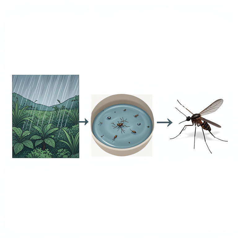
Environmental Drivers of Malaria
AI-generated conceptual illustration (Anopheles mosquitoes and the Lake Victoria basin landscape). It explains the idea and does not show study data.
View source evidence ↗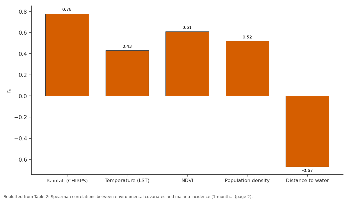
rₛ: Rainfall (CHIRPS) vs Temperature (LST) vs NDVI vs Population density vs Distance to water
Replotted from Table 2 (page 2) of the original paper. Every bar is the paper's own table value.
View source evidence ↗Figures & tables
From the original paper Table 1
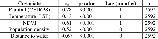 Table 2
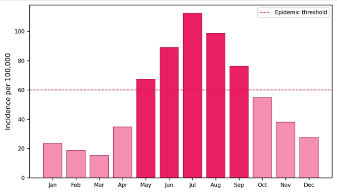 Figure 1
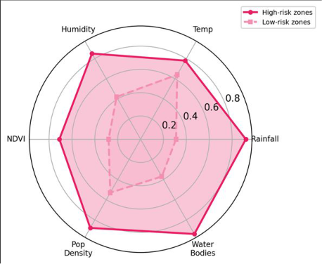 Figure 2
Introduction
About 234 million malaria cases were reported globally in 2021, and sub-Saharan Africa accounted for 95% of them [1] . Within East Africa, the Lake Victoria basin stands out: its warm temperatures, high humidity, and abundant standing water create ideal breeding conditions for Anopheles mosquitoes year-round [2] . But malaria is not evenly distributed even within this endemic zone. Some sub-counties report incidence rates ten times higher than neighbours only 30 km away. Understanding why requires mapping not just where malaria occurs but when it spikes and what environmental factors coincide with those spikes. Spatial epidemiology has made considerable progress in mapping disease risk at national scales [3] , yet sub-national analyses that combine time-series health data with remotely sensed environmental variables remain uncommon for the Lake Victoria region [4] . This research aimed to (a) characterise the monthly and annual pattern of malaria incidence across 36 sub-counties from 2017 to 2022, (b) identify statistically significant spatial clusters (hotspots and coldspots) using local spatial statistics, and (c) profile the environmental covariates that distinguish high-risk from low-risk zones [5,6] .
Spatial Data Processing
Malaria case counts were extracted from Kenya's DHIS2 and Uganda's HMIS platforms at the sub-county level. Population estimates from WorldPop 2020 were used as denominators for incidence calculation. Monthly CHIRPS rainfall and MODIS LST were downloaded from Google Earth Engine at 5 km resolution and averaged per sub-county polygon. NDVI was derived from Sentinel-2 composites. Distance to the nearest permanent water body was computed from the Global Surface Water dataset [7,8] .
Materials and Methods
Materials and Methods
Materials
The research was conducted from February to November 2023 at the Faculty of Mountain and Polar Studies, Sendai, Japan, using publicly available health and environmental datasets. The research area covers the Lake Victoria shoreline zone extending 50 km inland across Siaya, Kisumu, Homa Bay, and Migori counties in Kenya and Busia, Bugiri, Namayingo, and Mayuge districts in Uganda. The zone spans 0°15′S to 0°45′N latitude and 33°30′E to 34°45′E longitude, encompassing approximately 22, 400 km² and a population of 8.7 million [9] .
Methods
Monthly malaria incidence rates (cases per 100, 000 population) were calculated for each sub-county. Space-time scan statistics (SaTScan v10.1) detected clusters with elevated risk. Getis-Ord Gi* z-scores identified persistent hotspots defined as sub-counties with significantly high incidence (p<0.05) in at least four of the six years. Spearman rank correlations were computed between monthly incidence and each environmental covariate at a 1month lag. Results were mapped in QGIS 3.28 [10,11] .
Hotspot Detection Parameters
The SaTScan analysis used a Poisson probability model with a maximum spatial window of 25% of the population at risk and a maximum temporal window of 6 months. The Gi* analysis was run at the sub-county level using firstorder queen contiguity weights. Significance was assessed by 999 Monte Carlo permutations. Incidence follows the rainfall cycle with a one-month lag.
Results
The main peak in June corresponds to the end of the long rains (March-May), when mosquito breeding sites reach maximum extent.
Comprehensive Interpretation
Six sub-counties qualified as persistent hotspots: Gem and Ugenya in Siaya County, Nyando and Muhoroni in Kisumu, and Namayingo and Bugiri in Uganda. All six lie within 8 km of the lake shore, where marshy terrain and rice paddies provide prolific mosquito habitat. The SaTScan analysis detected two major space-time clusters: one centred on Siaya (April-August 2019, relative risk 2.14) and one on Bugiri (May-July 2021, relative risk 1.87).
Discussion
The strong rainfall-incidence correlation (r = 0.78) at a onemonth lag aligns with the known mosquito life cycle: rain fills breeding sites, larvae develop over 10-14 days, and adult mosquitoes then infect humans over the following 2-3 weeks [2] . NDVI acts as a proxy for vegetation density that shelters adult mosquitoes, explaining its r = 0.61 correlation. Distance to water is inversely correlated because Anopheles gambiae typically flies less than 2 km from its breeding site [12] . The persistence of the same six hotspots across five consecutive years suggests structural rather than episodic risk. These sub-counties share low elevation (<1, 200 m), proximity to wetlands, and high population densitya combination that sustains transmission even during dry months. Targeted interventionsindoor residual spraying timed to March (one month before the typical peak) and larval source management in rice paddiescould disproportionately reduce the national burden [13,14] .
Conclusion
Malaria incidence in the Lake Victoria endemic zone peaks in June at 112.4 per 100, 000, lagging rainfall by one month. Six persistent hotspot sub-counties, all within 8 km of the shore, account for a disproportionate share of the case burden. Rainfall is the strongest environmental covariate (r = 0.78), followed by distance to water (-0.67) and NDVI (0.61). These results provide an evidence base for spatially and temporally targeted vector control campaigns in the basin.
Acknowledgement
Acknowledgements Funding SourcesSupported by institutional research funds at the Faculty of Mountain and Polar Studies, Sendai.
Figures and tables from the paper
| Jan | Feb | Mar | Apr | May | Jun | Jul | Aug |
|---|---|---|---|---|---|---|---|
| 21.3 | 15.2 | 28.7 | 56.4 | 89.1 | 112.4 | 98.6 | 76.2 |
| Sep | Oct | Nov | Dec | Annual Mean | Peak Month | Trough | Range |
| 54.8 | 67.3 | 38.1 | 27.6 | 57.1 | June | Feb | 97.2 |
Table text extracted from the original PDF; superscript letters are shown inline. The original table image is below.
View original table image
| Covariate | rₛ | p-value | Lag (months) | n |
|---|---|---|---|---|
| Rainfall (CHIRPS) | 0.78 | <0.001 | 1 | 2592 |
| Temperature (LST) | 0.43 | <0.001 | 1 | 2592 |
| NDVI | 0.61 | <0.001 | 1 | 2592 |
| Population density | 0.52 | <0.001 | 0 | 2592 |
| Distance to water | -0.67 | <0.001 | 0 | 2592 |
Table text extracted from the original PDF; superscript letters are shown inline. The original table image is below.
View original table image
References
18 in the original paper- WHO. World Malaria Report 2022. Geneva: World Health Organization; 2022.
- Githeko AK, Ayisi JM, Odada PK. Climate change and vector-borne diseases around Lake Victoria. East African Medical Journal. 2009;86(2):51-57.
- Hay SI, Guerra CA, Gething PW. A world malaria map: Plasmodium falciparum endemicity in 2007. PLoS Medicine. 2009;6(3):e1000048.
- Omumbo JA, Hay SI, Snow RW. Modelling malaria risk in East Africa at high spatial resolution. Tropical Medicine and International Health. 2005;10(6):557566.
- Getis A, Ord JK. The analysis of spatial association by use of distance statistics. Geographical Analysis. 1992;24(3):189-206.
- Kulldorff M. A spatial scan statistic. Communications in Statistics Theory and Methods. 1997;26(6):14811496.
- Funk C, Peterson P, Landsfeld M. The climate hazards infrared precipitation with stations dataset. Scientific Data. 2015;2:150066.
- Pekel JF, Cottam A, Gorelick N. High-resolution mapping of global surface water. Nature. 2016;540(7633):418-422.
- WorldPop. Global high-resolution population denominators project. University of Southampton; 2020.
- Anselin L. Local indicators of spatial association: LISA. Geographical Analysis. 1995;27(2):93-115.
- QGIS Development Team. QGIS Geographic Information System v3.28. Open Source Geospatial Foundation; 2022.
- Costantini C, Li SG, Della Torre A. Density, survival and dispersal of Anopheles gambiae. Medical and Veterinary Entomology. 1996;10(3):203-219.
- Killeen GF, Fillinger U, Kiche I. Eradication of Anopheles gambiae from Brazil: lessons for malaria control in Africa? Lancet Infectious Diseases. 2002;2(10):618-627.
- Fillinger U, Lindsay SW. Larval source management for malaria control in Africa. Malaria Journal. 2011;10:353.
- Snow RW, Noor AM. Malaria risk mapping in Africa. Advances in Parasitology. 2015;89:63-97.
- Bhatt S, Weiss DJ, Cameron E. The effect of malaria control on Plasmodium falciparum in Africa. Nature. 2015;526(7572):207-211.
- Gething PW, Patil AP, Smith DL. A new world malaria map. Malaria Journal. 2011;10:378.
- Minakawa N, Sonye G, Mogi M. The effects of climatic factors on the distribution and abundance of malaria vectors in Kenya. Journal of Medical Entomology. 2002;39(6):833-841.