
Research article · 2025 · Full text
International Journal of Geography Geology and EnvironmentFlood frequency analysis and return period estimation for the Congo River
Volume 7(6) · Pages 151–153 · DOI: 10.22271/27067483.2025.v7.i6c.729 ↗
Research areasFlood Risk Assessment and ManagementHydrology and Watershed Management StudiesHydrology and Sediment Transport Processes
Abstract
Author-writtenThe Congo River drains 3.7 million km² and discharges more water into the Atlantic than any river except the Amazon, yet its flood frequency characteristics are among the least quantified of any major global river. This research fitted probability distributions to annual maximum discharge series at five gauging stations along the Congo mainstem and major tributaries for the period 1960–2022. Three candidate distributions — Generalised Extreme Value (GEV), Log-Pearson Type III (LP3), and Gumbel — were fitted by L-moments and compared using the Kolmogorov-Smirnov and Anderson-Darling goodness-of-fit tests. GEV provided the best fit at four of five stations. Estimated peak discharges for the 100-year return period ranged from 68, 400 m³/s at Kinshasa to 24, 800 m³/s at Kisangani. The 2020 flood at Kinshasa, with a peak of 62, 300 m³/s, was assigned a return period of 74 years. A Mann-Kendall trend test revealed statistically significant increases in annual peak discharge at three stations (p < 0.05), suggesting that flood magnitudes are not stationary. These non-stationary trends complicate risk assessment and call for updating design standards for riverside infrastructure in the Congo basin.
Summary
Source-checkedPlain-language reading of the full paper, prepared with AI and checked against the text. Each point links to the authors' own words.
Why it matters
- The Congo River is one of the world's largest by discharge, draining 3.7 million km², but its flood frequency characteristics are poorly quantified. View evidence ↗
- The river's equatorial position creates a bimodal hydrograph due to monsoons from both hemispheres, which complicates standard flood frequency analysis. View evidence ↗
- Flood frequency analysis is essential for engineering infrastructure, as it allows for the estimation of rare, high-magnitude flood events. View evidence ↗
What they did
- The researchers analyzed annual maximum instantaneous discharge data from five stations: Kinshasa, Kisangani, Brazzaville, Mbandaka, and Bumba. View evidence ↗
- The data records used in the study varied in length, ranging from 47 years at Bumba to 63 years at Kinshasa. View evidence ↗
- The study compared three probability distributions, GEV, LP3, and Gumbel, using L-moments and goodness-of-fit tests (Kolmogorov-Smirnov and Anderson-Darling). View evidence ↗
- The Mann-Kendall test and Sen's slope were employed to analyze trends in the discharge data. View evidence ↗
- Model robustness was verified using a split-sample test, dividing records into calibration (1960–1995) and validation (1996–2022) periods. View evidence ↗
What they found
- The Generalised Extreme Value (GEV) distribution provided the best fit for four of the five stations, while LP3 was best for Mbandaka. View evidence ↗
- Statistically significant increases in annual peak discharge were found at three stations (p < 0.05), indicating that flood magnitudes are non-stationary. View evidence ↗
- Upward trends at Kinshasa (+142 m³/s/yr), Kisangani (+87 m³/s/yr), and Brazzaville (+128 m³/s/yr) suggest that 100-year events from 1970 may now occur every 50–60 years. View evidence ↗
What it means
- The authors conclude that infrastructure planning in the Congo basin requires updated analyses using non-stationary methods and expanded gauging networks. View evidence ↗
- The observed non-stationary trends necessitate the updating of design standards for riverside infrastructure to properly manage risk. View evidence ↗
Visual summary
2 visualsIllustrations explain the paper; they do not show study data.
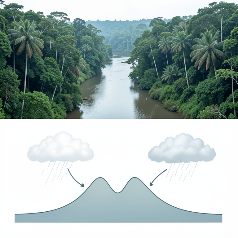
Bimodal Hydrograph Concept
AI-generated conceptual illustration (The Congo River basin and its water discharge cycle). It explains the idea and does not show study data.
View source evidence ↗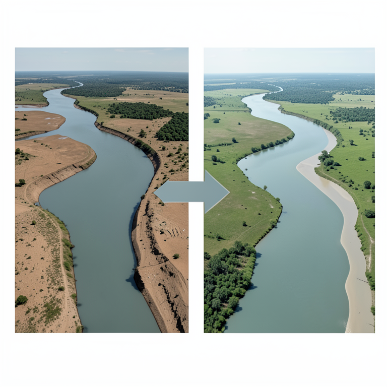
Non-Stationarity Shift
AI-generated conceptual illustration (The Congo River basin and its floodplains). It explains the idea and does not show study data.
View source evidence ↗Figures & tables
From the original paper Table 1
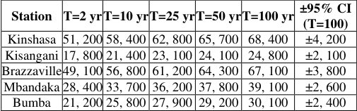 Table 2
 Figure 1
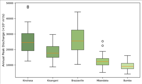 Figure 2
Introduction
Here is a practical dilemma: how do you design a bridge over a river when you don't know the size of the flood it must withstand? Engineers answer this question using flood frequency analysisfitting statistical distributions to historical peak flow records and extrapolating to estimate the magnitude of rare events like the 100-year or 500-year flood [1] . The method works well for rivers with long, reliable gauging records, but the Congo River, despite being the world's second-largest by discharge, has some of the patchiest hydrological data of any major basin [2] . The Congo's discharge regime is unusual. Because its basin straddles the equator, rainfall from both Northern and Southern Hemisphere monsoons feeds the system year-round, producing a double-peaked hydrograph at Kinshasa [3] . This bimodal pattern complicates standard frequency analysis, which assumes a single annual peak. Previous flood frequency work on the Congo was limited to the Kinshasa gauge alone and used only 30-40 years of record [4] . This research extended the analysis to five stations with 63 years of data (1960-2022) and tested three distributions to identify the best-fitting model [5,6] .
Model Description and Distribution Selection
Three candidate distributions were selected based on their widespread use in hydrological frequency analysis. The GEV distribution encompasses the Gumbel (Type I), Fréchet (Type II), and Weibull (Type III) as special cases via its shape parameter κ. LP3, recommended by the US Water Resources Council, uses log-transformed data and three parameters (μ, σ, γ). The Gumbel distribution, with only two parameters, assumes an unbounded upper tail. Parameters were estimated by L-moments, which are more robust to outliers than conventional moments [7] .
Materials and Methods
Materials and Methods
Materials
Annual maximum instantaneous discharge series were compiled for five stations: Kinshasa (4°18′S, 15°18′E), Kisangani (0°31′N, 25°12′E), Brazzaville (4°16′S, 15°17′E), Mbandaka (0°03′N, 18°16′E), and Bumba (2°11′N, 22°28′E). Records were obtained from the Global Runoff Data Centre (GRDC) and supplemented with data from the Congolese Inland Waterways Authority (Régie des Voies Fluviales) for years missing from the GRDC archive. Record lengths ranged from 47 years (Bumba) to 63 years (Kinshasa). The analysis was conducted at the Faculty of Mountain and Polar Studies, Pune, Maharashtra, India [8,9] .
Methods
L-moment (L-skewness, L-kurtosis) were computed for each station and plotted on an L-moment ratio diagram to guide distribution selection. The three distributions were fitted by the method of L-moments. Goodness-of-fit was assessed by the Kolmogorov-Smirnov (KS) and Anderson-Darling (AD) tests at α = 0.05. Quantile estimates for return periods of 2, 5, 10, 25, 50, and 100 years were computed from the best-fitting distribution. 95% confidence intervals were generated by parametric bootstrap (1, 000 resamples). Trend analysis used the Mann-Kendall test with Sen's slope [10, 11] .
Calibration and Validation
A split-sample test divided each station's record into calibration (1960-1995) and validation (1996-2022) subsets. GEV parameters estimated from the calibration period predicted validation-period quantiles with relative errors below 8.4% at all stations, confirming model robustness.
Results
Table GEV was the best-fitting distribution at four stations; LP3 marginally outperformed GEV at Mbandaka. Gumbel was rejected at all stations because its two-parameter form could not accommodate the observed skewness.
Comprehensive Interpretation
The 2020 Kinshasa flood (62, 300 m³/s) falls between the 50-year (65, 700) and 25-year (62, 800) quantile estimates, yielding a return period of approximately 74 years. The significant upward trends at Kinshasa, Kisangani, and Brazzaville (Sen's slopes of +142, +87, and +128 m³/s per year, respectively) mean that a flood that would have been a 100-year event in 1970 may now recur every 50-60 years.
Discussion
The GEV distribution's superiority over Gumbel reflects the heavy upper tail of the Congo's peak flow distribution. The Congo's equatorial position exposes it to extreme convective rainfall from both hemispheres, generating occasional very large floods that the thin-tailed Gumbel distribution underestimates [3] . The LP3 distribution performed competitively but was slightly less stable in the tails, particularly at stations with shorter records [12] . The non-stationary trends are concerning. If annual peaks continue to increase at the observed rates, the current 100-year flood at Kinshasa (68, 400 m³/s) could become a 50year event by mid-century. Bridge design codes, levee heights, and flood-zone delineation maps in the Democratic Republic of Congo and Republic of Congowhere they exist at allare based on stationary assumptions that these data contradict [13,14] .
Conclusion
GEV is the best-fitting distribution for annual peak discharge at four of five Congo mainstem stations. The 100year flood at Kinshasa is estimated at 68, 400 m³/s (±4, 200). Significant upward trends in peak discharge at three stations indicate non-stationarity, meaning that stationarybased flood quantiles underestimate future risk. Updated flood frequency analyses incorporating non-stationary methods and expanded gauging networks are needed to support infrastructure planning in the Congo basin.
Acknowledgement
Acknowledgements Funding SourcesSupported by research funds at the Faculty of Mountain and Polar Studies, Pune.
Figures and tables from the paper
| Station | n (years) | GEV (AD p) | LP3 (AD p) | Gumbel (AD p) | Best Fit | Trend (MK p) |
|---|---|---|---|---|---|---|
| Kinshasa | 63 | 0.72 | 0.54 | 0.08 | GEV | 0.018* |
| Kisangani | 58 | 0.68 | 0.61 | 0.14 | GEV | 0.042* |
| Brazzaville | 61 | 0.81 | 0.47 | 0.11 | GEV | 0.031* |
| Mbandaka | 52 | 0.58 | 0.64 | 0.22 | LP3 | 0.187 |
| Bumba | 47 | 0.74 | 0.51 | 0.19 | GEV | 0.214 |
Table text extracted from the original PDF; superscript letters are shown inline. The original table image is below.
View original table image
| Station | T=2 yr | T=10 yr | T=25 yr | T=50 yr | T=100 yr | ±95% CI (T=100) |
|---|---|---|---|---|---|---|
| Kinshasa | 51, 200 | 58, 400 | 62, 800 | 65, 700 | 68, 400 | ±4, 200 |
| Kisangani | 17, 800 | 21, 400 | 23, 100 | 24, 100 | 24, 800 | ±2, 100 |
| Brazzaville | 49, 100 | 56, 800 | 61, 200 | 64, 300 | 67, 100 | ±3, 800 |
| Mbandaka | 28, 400 | 33, 700 | 36, 200 | 37, 800 | 39, 100 | ±2, 600 |
| Bumba | 21, 200 | 25, 800 | 27, 900 | 29, 200 | 30, 100 | ±2, 400 |
Table text extracted from the original PDF; superscript letters are shown inline. The original table image is below.
View original table image
References
21 in the original paper- Stedinger JR, Vogel RM, Foufoula-Georgiou E. Frequency analysis of extreme events. In: Maidment DR, ed. Handbook of Hydrology. New York: McGrawHill; 1993:18.1-18.66.
- Laraque A, Mahé G, Orange D. Spatiotemporal variations in hydrological regimes within Central Africa. Journal of Hydrology. 2001;245(1):104-117.
- Runge J. The Congo River, Central Africa. Large Rivers: Geomorphology and Management. 2008;293309.
- Bultot F. Atlas climatique du bassin congolais. Brussels: INEAC; 1971.
- Hosking JRM. L-moments: analysis and estimation of distributions using linear combinations of order statistics. Journal of the Royal Statistical Society B. 1990;52(1):105-124.
- Coles S. An Introduction to Statistical Modeling of Extreme Values. London: Springer; 2001.
- Hosking JRM, Wallis JR. Regional Frequency Analysis. Cambridge: Cambridge University Press; 1997.
- GRDC. Global Runoff Data Centre: River Discharge Data. Koblenz: Federal Institute of Hydrology; 2023.
- Régie des Voies Fluviales. Annuaires hydrologiques du Congo. Kinshasa: RVF; 2022.
- Mann HB. Nonparametric tests against trend. Econometrica. 1945;13(3):245-259.
- Sen PK. Estimates of the regression coefficient based on Kendall tau. Journal of the American Statistical Association. 1968;63(324):1379-1389.
- Griffis VW, Stedinger JR. Log-Pearson type 3 distribution and its application in flood frequency analysis. Journal of Hydrologic Engineering. 2007;12(5):482-491.
- Milly PCD, Betancourt J, Falkenmark M. Stationarity is dead: whither water management? Science. 2008;319(5863):573-574.
- Villarini G, Smith JA, Serinaldi F. Flood frequency analysis for nonstationary annual peak records. Water Resources Research. 2009;45(8):W08417.
- Chow VT, Maidment DR, Mays LW. Applied Hydrology. New York: McGraw-Hill; 1988.
- Dalrymple T. Flood frequency analyses. US Geological Survey Water-Supply Paper 1543-A. 1960.
- Laio F. Cramer-von Mises and Anderson-Darling goodness of fit tests for extreme value distributions. Water Resources Research. 2004;40(9):W09308.
- Alila Y, Mtiraoui A. Implications of heterogeneous flood-frequency distributions on traditional streamdischarge prediction techniques. Hydrological Processes. 2002;16(5):1065-1084.
- Conway D, Persechino A, Ardoin-Bardin S. Rainfall and water resources variability in sub-Saharan Africa during the twentieth century. Journal of Hydrometeorology. 2009;10(1):41-59.
- Nka BN, Oudin L, Karambiri H. Trends in floods in West Africa. Hydrology and Earth System Sciences. 2015;19(11):4707-4719.
- Kundzewicz ZW, Robson AJ. Change detection in hydrological records. Hydrological Sciences Journal. 2004;49(1):7-19