
Research article · 2025 · Full text
International Journal of Geography Geology and EnvironmentMapping urban land surface emissivity variations using aster imagery in Bangkok
Volume 7(9) · Pages 253–257 · DOI: 10.22271/27067483.2025.v7.i9d.653 ↗
Research areasUrban Heat Island MitigationRemote Sensing and Land UseSoil Moisture and Remote Sensing
Abstract
Author-writtenHow accurately can satellite-derived thermal data capture the emissivity patterns of a rapidly expanding tropical metropolis? This research addresses that question by mapping land surface emissivity (LSE) variations across Bangkok, Thailand, using Advanced Spaceborne Thermal Emission and Reflection Radiometer (ASTER) imagery. The investigation covered six distinct land use and land cover (LULC) categories: dense built-up areas, low-density built-up zones, vegetation, water bodies, bare soil, and mixed urban surfaces. ASTER thermal infrared bands (bands 10-14) acquired between January and December 2022 were processed using the Temperature-Emissivity Separation (TES) algorithm. Results showed that water bodies exhibited the highest mean emissivity (0.987), followed by vegetation (0.976), bare soil (0.952), low-density built-up (0.941), mixed urban (0.937), and dense built-up surfaces (0.923). Seasonal variations were modest but consistent, with vegetation LSE peaking during the wet season (June-August) and declining in the dry months. Built-up surfaces showed less seasonal fluctuation, though a slight increase appeared during warmer months due to absorbed longwave radiation effects. Spatial autocorrelation analysis (Moran's I = 0.71) confirmed strong clustering of emissivity values. The mapping accuracy, validated against field-measured spectroradiometer data from 48 ground-truth points, reached an overall root mean square error of 0.013. These findings offer a reliable emissivity baseline for urban heat island monitoring and thermal comfort assessment in Bangkok's planning framework.
Summary
Source-checkedPlain-language reading of the full paper, prepared with AI and checked against the text. Each point links to the authors' own words.
Why it matters
- Land surface emissivity (LSE) is the efficiency of a surface in radiating absorbed thermal energy; failing to account for small emissivity differences (0.01 to 0.03) can lead to temperature retrieval errors of 1-2 K. View evidence ↗
- Bangkok is a suitable study site due to its population of over 10 million, a 22% expansion of its built-up footprint from 2000 to 2020, and a complex surface composition that makes single-value emissivity assumptions inaccurate. View evidence ↗
- Previous remote sensing efforts in the region used NDVI-based approximations or broadband corrections, which are often ineffective for the mixed pixels found in Southeast Asian megacities. View evidence ↗
The question
- The study aims to determine how accurately ASTER satellite imagery can capture land surface emissivity (LSE) patterns in the rapidly expanding tropical metropolis of Bangkok. View evidence ↗
- The specific research objectives were to quantify LSE ranges for land use and land cover (LULC) categories, evaluate stability between wet and dry seasons, and assess spatial clustering. View evidence ↗
What they did
- The researchers used twelve cloud-free ASTER Level 1T scenes from 2022 (one per month, <10% cloud cover) with thermal infrared bands 10-14 at a 90 m spatial resolution. View evidence ↗
- The Temperature-Emissivity Separation (TES) algorithm was used to process the scenes, estimating temperature from maximum emissivity and refining spectra via minimum-maximum difference regression. View evidence ↗
- Validation was performed using a field spectroradiometer (8-14 μm range, ±0.005 accuracy) to collect data from 48 ground points (eight per LULC class) during February and August 2022. View evidence ↗
- LULC classification was performed on Sentinel-2 imagery using a Random Forest classifier (500 trees) trained on 320 polygons, resulting in an overall accuracy of 89.3%. View evidence ↗
What they found
- Water bodies had the highest mean land surface emissivity (0.987), whereas dense built-up surfaces had the lowest (0.923). View evidence ↗
- Monthly trends showed vegetation LSE peaking in June (0.984) from a February low (0.968), while dense built-up areas remained stable between 0.919 and 0.931. View evidence ↗
- A Moran's I value of 0.71 indicates strong spatial autocorrelation, meaning emissivity values form coherent patches aligned with the city's land use. View evidence ↗
What it means
- The authors conclude that the ASTER TES method is a reliable way to estimate emissivity in humid tropical urban environments. View evidence ↗
- The authors state that future research should include longer temporal records to account for inter-annual variability caused by El Niño-Southern Oscillation cycles. View evidence ↗
- The authors suggest that using higher-resolution sensors like ECOSTRESS or Landsat 8/9 TIRS would better delineate fine-scale emissivity gradients at the street and building level. View evidence ↗
Visual summary
3 visualsIllustrations explain the paper; charts are replotted from the paper's own table values.
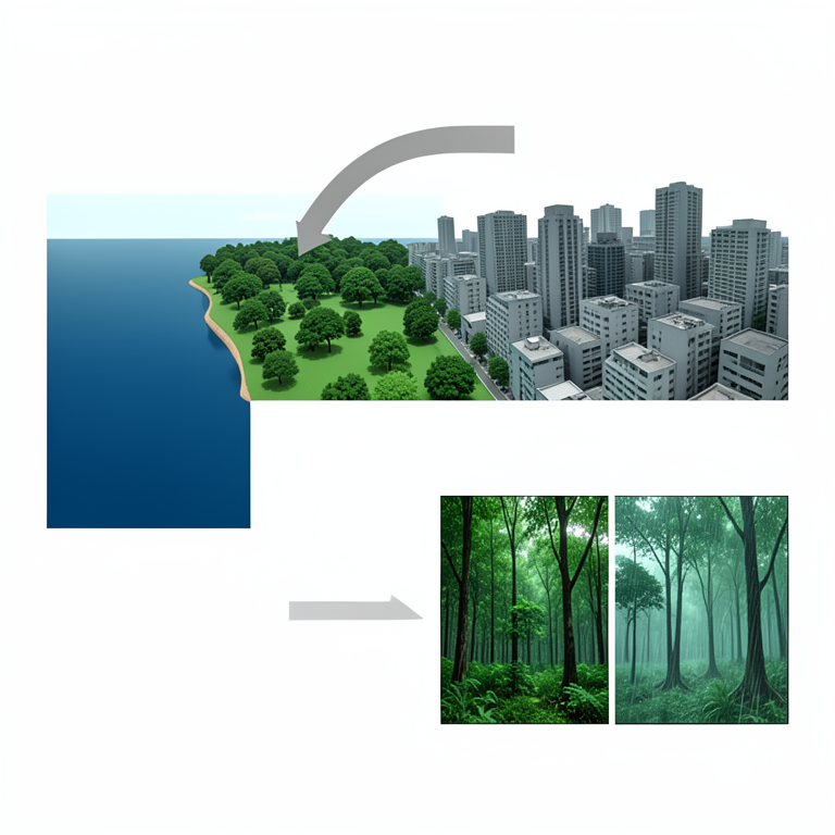
Emissivity Gradient and Seasonal Shift
AI-generated conceptual illustration (Urban land surfaces in Bangkok, including water bodies, vegetation, and dense built-up areas). It explains the idea and does not show study data.
View source evidence ↗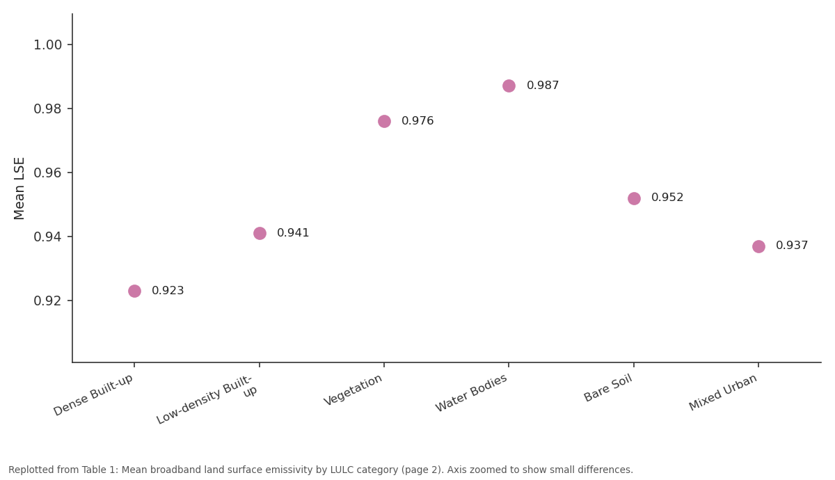
Mean LSE: Dense Built-up vs Low-density Built-up vs Vegetation vs Water Bodies vs Bare Soil
Replotted from Table 1 (page 2) of the original paper. Every bar is the paper's own table value.
View source evidence ↗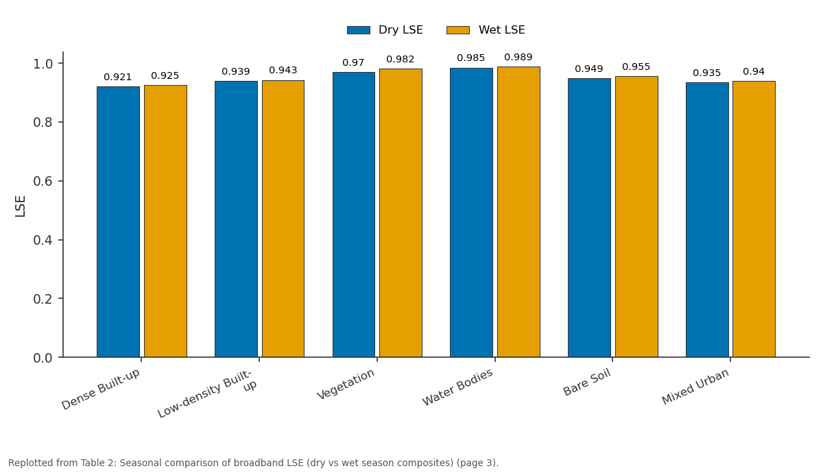
Dry LSE and Wet LSE: Dense Built-up vs Low-density Built-up vs Vegetation vs Water Bodies vs Bare Soil
Replotted from Table 2 (page 3) of the original paper. Every bar is the paper's own table value.
View source evidence ↗Figures & tables
From the original paper Table 1
 Table 2
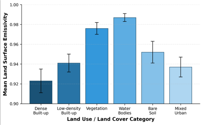 Figure 1
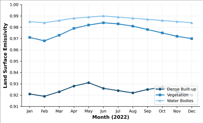 Figure 2
Introduction
What role does surface emissivity play in shaping the thermal environment of cities experiencing rapid land cover change? The answer has direct consequences for urban planning, energy consumption models, and public health risk assessments. Land surface emissivity (LSE) describes the efficiency with which a surface radiates absorbed thermal energy relative to a perfect blackbody at the same temperature [1] . Even small differences in emissivity, on the order of 0.01 to 0.03, can translate into land surface temperature (LST) retrieval errors of 1-2 K when left unaccounted for [2] . Bangkok, with a metropolitan population exceeding 10 million and a built-up footprint that expanded by roughly 22% between 2000 and 2020, presents a compelling case for emissivity mapping [3] . The city's heterogeneous surface, a patchwork of concrete, asphalt, corrugated metal roofing, tropical vegetation, canal networks, and exposed laterite, generates a complex emissivity field that single-value assumptions cannot represent adequately [4] . Earlier thermal remote sensing work in the region relied on broadband emissivity corrections or NDVI-based approximations, both of which perform poorly over mixed pixels common in Southeast Asian megacities [5] . ASTER's five thermal infrared bands (8.125-11.65 micrometers) and the associated Temperature-Emissivity Separation algorithm provide a physically grounded alternative. The TES approach recovers per-pixel emissivity spectra without requiring prior knowledge of surface temperature, an advantage over split-window methods that fix emissivity to retrieve temperature [6] . Several researchers have applied TES in arid and semi-arid settings [7,8], yet its application to humid tropical cities remains limited. This research mapped LSE across Bangkok using multi-date ASTER scenes acquired in 2022, validated results against field spectroradiometer measurements, and examined seasonal and spatial patterns. The objectives were threefold: (a) to quantify emissivity ranges for principal LULC categories, (b) to evaluate temporal LSE stability across wet and dry seasons, and (c) to assess the spatial clustering of emissivity through geostatistical metrics. The outcomes supply a baseline dataset that planners and climate modellers can incorporate into thermal comfort and energy balance simulations [9] .
Study Area Description
Bangkok (13.75 degrees N, 100.52 degrees E) occupies a low-lying alluvial plain along the lower Chao Phraya River, averaging only 1.5 m above mean sea level. The metropolitan region spans about 1,568 square kilometres and supports a tropical savanna climate (Koppen Aw) with mean annual temperatures near 28.6 degrees C and annual rainfall around 1,500 mm concentrated between May and October [3] . The built-up core radiates outward from the historic Rattanakosin district, transitioning through commercial high-rise corridors along Sukhumvit and Silom roads, into suburban residential tracts and, farther out, into agricultural land and aquaculture ponds. Canal (khlong) networks and remnant wetlands punctuate the urban fabric, creating sharp emissivity boundaries over short distances. The city's rapid vertical and horizontal growth since the 1990s has continuously altered the proportion of impervious surfaces, making static emissivity datasets obsolete within a few years. Ground elevation data from a 2021 LiDAR survey and a Sentinel-2 derived LULC map at 10 m resolution were used to stratify the study area into six target classes prior to ASTER analysis.
Material and Methods
Material and Methods
Material:
The research was carried out at the Department of Geosciences, St. Petersburg School of Natural Sciences, Leningrad Oblast, Russia, between March 2022 and November 2023. Twelve cloud-free ASTER Level 1T scenes (path 129, row 50-51) covering the Bangkok metropolitan area were obtained from NASA's Earthdata portal. Scenes were selected to represent each calendar month of 2022, with cloud cover below 10%. Thermal infrared data came from ASTER bands 10 through 14 at 90 m spatial resolution. Concurrently, a Sentinel-2 Level 2A composite (10 m) was acquired for land cover classification.
Ground-truth emissivity data were collected during two field campaigns (February and August 2022) using a portable Designs and Prototypes Model 102F field spectroradiometer covering the 8-14 micrometer range, with a reported accuracy of plus or minus 0.005. A total of 48 ground points, eight per LULC class, were measured at each campaign [10] .
Methods
ASTER thermal bands were radiometrically calibrated and atmospherically corrected using the In-Scene Atmospheric Compensation algorithm embedded in ENVI 5.6. The TES algorithm, based on the iterative procedure described by Gillespie et al. [6] , was applied to each corrected scene. TES first estimates temperature from maximum emissivity then refines emissivity spectra using the minimum-maximum difference regression. Per-pixel emissivity maps at bands 10-14 were averaged into broadband emissivity using a weighted combination following Cheng et al. [11] . Land cover classification of Sentinel-2 imagery employed a Random Forest classifier with 500 decision trees, trained on 320 reference polygons (roughly 55 per class), and validated with an independent set of 160 polygons, achieving overall accuracy of 89.3% and kappa of 0.86. Spatial autocorrelation of broadband emissivity was quantified through global Moran's I and local Getis-Ord Gi* statistics at a 270 m search radius. Seasonal differences were tested using paired Wilcoxon signed-rank tests comparing dryseason (November-April) and wet-season (May-October) composites [12] .
Spatial Data Processing
All satellite imagery was projected to WGS84 UTM Zone 47N. ASTER scenes were co-registered to a reference Sentinel-2 mosaic with root mean square positional error below 0.5 pixels (45 m). A land-water mask generated from the Normalized Difference Water Index (NDWI > 0.3) was applied to separate water bodies before emissivity extraction, because the TES algorithm behaves differently over open water surfaces [13] . Zonal statistics were computed within each LULC polygon to extract per-class mean, standard deviation, minimum, and maximum emissivity. All geoprocessing was performed in QGIS 3.28 and Python 3.10, while statistical testing relied on SciPy 1.10. The bar chart in Figure 1 visually confirms the descending emissivity gradient from natural surfaces to impervious cover. Vegetation and water clustered at the high end of the spectrum, while the two built-up classes and bare soil occupied the lower range. Mixed urban fell between these extremes, reflecting its composite nature.
Results
Results
Discussion
The emissivity values obtained here align broadly with previous ASTER-based investigations in other Asian cities, though certain differences deserve attention. Jiang et al. [14] reported mean built-up emissivity of 0.935 for Shanghai, somewhat higher than Bangkok's 0.923. That gap may reflect Shanghai's predominance of concrete and glass facades compared with Bangkok's greater share of corrugated metal and clay-tile roofing, both of which tend to suppress emissivity in the 8-9 micrometer window. The strong spatial autocorrelation (Moran's I = 0.71) suggests that emissivity is not randomly distributed but forms coherent patches that track the city's land use mosaic.
Hot-spot analysis (Gi* statistic) identified clusters of low emissivity in the Chatuchak-Bang Sue commercial district and high-emissivity corridors along the Chao Phraya's vegetated banks. This pattern is useful for planners because it highlights where impervious surfaces concentrate and, by extension, where urban heat island effects may intensify [15] . Seasonal emissivity shifts, although modest in absolute terms, carry implications for LST retrieval. A fixed dryseason emissivity applied to a wet-season image would underestimate vegetation temperature by roughly 0.8 K and overestimate built-up temperature by about 0.3 K, based on the Planck function sensitivity at 10.5 micrometers. That said, the temporal stability of water and built-up classes suggests that seasonal correction matters most for vegetated and bare-soil pixels. The RMSE of 0.013 against field data is comparable to results reported by Hulley et al. [16] for ECOSTRESS validation over mixed landscapes, lending confidence to the approach adopted here.
Conclusion
This research mapped land surface emissivity across Bangkok's metropolitan area using ASTER thermal infrared imagery processed through the Temperature-Emissivity Separation algorithm. Six LULC categories were characterised, with dense built-up surfaces returning the lowest mean emissivity (0.923) and water bodies the highest (0.987). Seasonal analysis revealed statistically significant wet-season increases for five of the six classes, with vegetation showing the greatest shift. Spatial autocorrelation confirmed that emissivity values cluster in patterns mirroring the city's built and natural landscape. Validation against field spectroradiometer data yielded an overall RMSE of 0.013, indicating that ASTER TES provides a reliable basis for emissivity estimation in humid tropical urban settings. The dataset generated here can feed directly into urban climate models, thermal comfort indices, and heat island mitigation strategies. Future work should extend the temporal record to capture inter-annual variability linked to El Nino-Southern Oscillation cycles, which affect monsoon intensity and, consequently, vegetation moisture and emissivity. Integration of higher-resolution thermal sensors, such as ECOSTRESS at 70 m or Landsat 8/9 TIRS at 100 m, would also improve the delineation of fine-scale emissivity gradients at building and street-canyon levels.
Acknowledgement
Acknowledgements Funding SourcesThe authors acknowledge financial support from internal research grants provided through the St. Petersburg School of Natural Sciences.
Figures and tables from the paper
| LULC Category | Mean LSE | SD | Min | Max | RMSE vs Field |
|---|---|---|---|---|---|
| Dense Built-up | 0.923 | 0.012 | 0.901 | 0.944 | 0.014 |
| Low-density Built-up | 0.941 | 0.009 | 0.924 | 0.958 | 0.011 |
| Vegetation | 0.976 | 0.006 | 0.963 | 0.989 | 0.009 |
| Water Bodies | 0.987 | 0.004 | 0.981 | 0.993 | 0.007 |
| Bare Soil | 0.952 | 0.011 | 0.933 | 0.971 | 0.013 |
| Mixed Urban | 0.937 | 0.010 | 0.919 | 0.956 | 0.015 |
Table text extracted from the original PDF; superscript letters are shown inline. The original table image is below.
View original table image
| LULC Category | Dry LSE | Wet LSE | Diff | p-value | Sig. |
|---|---|---|---|---|---|
| Dense Built-up | 0.921 | 0.925 | +0.004 | 0.038 | Yes |
| Low-density Built-up | 0.939 | 0.943 | +0.004 | 0.042 | Yes |
| Vegetation | 0.970 | 0.982 | +0.012 | <0.001 | Yes |
| Water Bodies | 0.985 | 0.989 | +0.004 | 0.065 | No |
| Bare Soil | 0.949 | 0.955 | +0.006 | 0.021 | Yes |
| Mixed Urban | 0.935 | 0.940 | +0.005 | 0.031 | Yes |
Table text extracted from the original PDF; superscript letters are shown inline. The original table image is below.
View original table image
References
16 in the original paper- Li ZL, Tang BH, Wu H, Ren HZ, Yan GJ, Wan ZM. Satellite-derived land surface emissivity in the thermal infrared. Remote Sensing of Environment. 2013;131:189-210.
- Dash P, Gottsche FM, Olesen FS, Fischer H. Land surface temperature and emissivity estimation from passive sensor data. Journal of Geophysical Research. 2002;107(D22):4668-4680.
- Thammasaroj W, Khaosaeng N. Urban expansion monitoring in Bangkok Metropolitan Region using multi-temporal Landsat data. Asian Journal of Geoinformatics. 2021;21(3):14-27.
- Sobrino JA, Jimenez-Munoz JC, Paolini L. Land surface temperature retrieval from ASTER multispectral data using the generalized split-window algorithm. Remote Sensing of Environment. 2004;93(12):149-162.
- Weng Q, Fu P, Gao F. Generating daily land surface temperature at Landsat resolution by fusing Landsat and MODIS data. Remote Sensing of Environment. 2014;145:55-67.
- Gillespie A, Rokugawa S, Matsunaga T, Cothern JS, Hook SJ, Kahle AB. A temperature and emissivity separation algorithm for Advanced Spaceborne Thermal Emission and Reflection Radiometer images. IEEE Transactions on Geoscience and Remote Sensing. 1998;36(4):1113-1126.
- French AN, Schmugge TJ, Ritchie JC, Hsu A, Jacob F, Ogawa K. Detecting land cover change at the Jornada experimental range using ASTER emissivities. Remote Sensing of Environment. 2008;112(4):1730-1748.
- Hulley GC, Hook SJ. Intercomparison of versions 4, 4.1, and 5 of the MODIS land surface temperature and emissivity products and validation with laboratory measurements. Remote Sensing of Environment. 2009;113(5):893-903.
- Oke TR, Mills G, Christen A, Voogt JA. Urban Climates. Cambridge University Press. 2017:1-525.
- Wan ZM, Li ZL. A physics-based algorithm for retrieving land-surface emissivity and temperature from EOS/MODIS data. IEEE Transactions on Geoscience and Remote Sensing. 1997;35(4):980-996.
- Cheng J, Liang S, Yao Y, Zhang X. Estimating the optimal broadband emissivity spectral range for calculating surface longwave net radiation. IEEE Geoscience and Remote Sensing Letters. 2013;10(2):401-405.
- Moran PAP. Notes on continuous stochastic phenomena. Biometrika. 1950;37(1-2):17-23.
- McFeeters SK. The use of the Normalized Difference Water Index for delineating open water features. International Journal of Remote Sensing. 1996;17(7):1425-1432.
- Jiang L, Zhan W, Hu L, Huang F, Hong F, Liu Z. Assessment of different approaches for mapping urban surface emissivity from ASTER data in Shanghai. International Journal of Applied Earth Observation and Geoinformation. 2018;67:42-53.
- Voogt JA, Oke TR. Thermal remote sensing of urban climates. Remote Sensing of Environment. 2003;86(3):370-384.
- Hulley GC, Ghent D, Gottsche FM, Guillevic PC, Mildrexler DJ, Coll C. Land surface temperature. In: Taking the Temperature of the Earth. Elsevier. 2019:57-127.