
Research article · 2025 · Full text
International Journal of Geography Geology and EnvironmentAtmospheric boundary layer dynamics and pollution dispersion modeling in Mexico city
Volume 7(5) · Pages 89–93 · DOI: 10.22271/27067483.2025.v7.i5b.596 ↗
Research areasAtmospheric chemistry and aerosolsAir Quality Monitoring and ForecastingWind and Air Flow Studies
Abstract
Author-writtenWhile many of the world's megacities sprawl across coastal plains where sea breezes help flush pollutants, Mexico City sits trapped in a high-altitude basin surrounded by volcanic mountains—a geography that turns the atmospheric boundary layer into a lid on the city's air. This research examined how boundary layer height (BLH) dynamics control the dispersion of fine particulate matter (PM2.5) across the Mexico City Metropolitan Area (MCMA). Radiosonde profiles and ceilometer backscatter data from five monitoring stations were analysed for the period January-December 2022, alongside concurrent surface-level PM2.5 measurements from 24 air quality stations. The Gaussian plume dispersion model AERMOD was parameterised with local meteorological inputs to simulate pollution concentration fields under varying BLH regimes. Results showed a strong inverse relationship between BLH and surface PM2.5 concentrations (r = −0.78, p<0.01). Morning BLH values averaged 387 m, trapping pollutants near the surface with PM2.5 peaks reaching 148 μg/m³, while afternoon convective growth expanded the boundary layer to 2,640 m and diluted concentrations to 27 μg/m³. The AERMOD simulations reproduced observed spatial patterns with an index of agreement of 0.81. Mobile sources contributed 41.8% of the basin's PM2.5 burden. These results highlight the dominant role of diurnal boundary layer cycling in determining when and where pollution episodes occur, and they offer guidance for short-term air quality forecasting in high-altitude enclosed basins.
Summary
Source-checkedPlain-language reading of the full paper, prepared with AI and checked against the text. Each point links to the authors' own words.
Why it matters
- Mexico City's geography, characterized by a high-altitude basin surrounded by volcanic mountains, creates an atmospheric boundary layer that acts as a lid, trapping pollutants. View evidence ↗
- The city's basin geometry limits horizontal ventilation, and intense solar heating drives a daily cycle in boundary layer height, which determines how well surface emissions are diluted. View evidence ↗
- Previous pollution models in Mexico City often relied on estimated boundary layer height (BLH) from energy balance calculations, which can lead to systematic errors during winter thermal inversions. View evidence ↗
The question
- The study aimed to examine how the dynamics of boundary layer height control the dispersion of fine particulate matter (PM2.5) in the Mexico City Metropolitan Area. View evidence ↗
What they did
- The study analyzed radiosonde and ceilometer data from five stations and PM2.5 measurements from 24 stations throughout 2022. View evidence ↗
- The AERMOD dispersion model (version 22112) was used on a 50 x 50 km domain with a 1-km receptor grid and 30-m DEM terrain elevations. View evidence ↗
- Simulations were conducted for 12 representative days, one for each month of 2022, covering various seasonal conditions. View evidence ↗
- The relationship between hourly BLH and surface PM2.5 was analyzed using Pearson correlation and exponential regression on approximately 8,400 paired observations. View evidence ↗
What they found
- A strong inverse relationship was found between boundary layer height and surface PM2.5 concentrations (r = -0.78, p < 0.01). View evidence ↗
- During the dry season, morning BLH averaged 387 m with PM2.5 peaks of 148 μg/m³, while afternoon BLH grew to 2,640 m, diluting concentrations to 27 μg/m³. View evidence ↗
- AERMOD simulations successfully reproduced observed spatial pollution patterns with an index of agreement of 0.81. View evidence ↗
- Mobile sources were the primary contributor to PM2.5 at 41.8%, followed by industrial emissions (23.4%) and residential combustion (16.7%). View evidence ↗
- Using default AERMET estimates instead of observed BLH increased the Normalized Mean Square Error (NMSE) by 37%, demonstrating the importance of direct measurements. View evidence ↗
- Model performance was highest during dry-season inversions (d = 0.86) and lowest during wet-season convective days (d = 0.74) due to thunderstorm outflows disrupting Gaussian assumptions. View evidence ↗
What it means
- The authors recommend integrating real-time ceilometer BLH measurements into AERMOD for better forecasting and implementing time-differentiated traffic restrictions during morning hours. View evidence ↗
- The authors state that future work should expand the ceilometer network to the southern and western basin and evaluate Lagrangian particle dispersion models for convective episodes. View evidence ↗
Visual summary
3 visualsIllustrations explain the paper; charts are replotted from the paper's own table values.
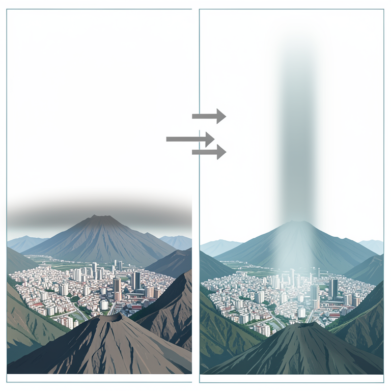
Diurnal Boundary Layer Cycle
AI-generated conceptual illustration (Mexico City in a mountain basin). It explains the idea and does not show study data.
View source evidence ↗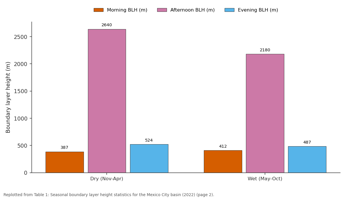
Morning BLH (m) and Afternoon BLH (m) and more: Dry (Nov-Apr) vs Wet (May-Oct)
Replotted from Table 1 (page 2) of the original paper. Every bar is the paper's own table value.
View source evidence ↗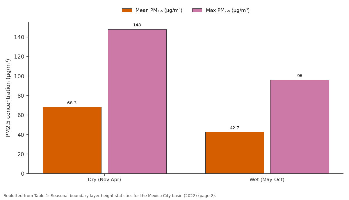
Mean PM₂.₅ (μg/m³) and Max PM₂.₅ (μg/m³): Dry (Nov-Apr) vs Wet (May-Oct)
Replotted from Table 1 (page 2) of the original paper. Every bar is the paper's own table value.
View source evidence ↗Figures & tables
From the original paper Table 1
 Table 2
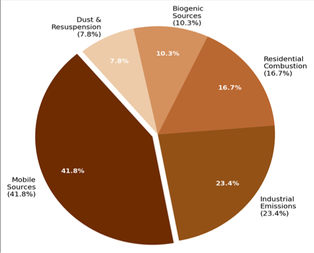 Figure 1
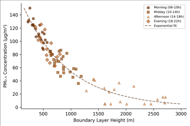 Figure 2
Introduction
Coastal megacities like Mumbai and Shanghai benefit from onshore winds that carry pollution out to sea each afternoon, but Mexico City enjoys no such relief. Sitting at 2,240 m elevation in a semi-enclosed basin ringed by mountains exceeding 5,000 m, the capital of Mexico has battled poor air quality for decades [1] . The basin geometry restricts horizontal ventilation, while the high altitude and subtropical latitude produce intense solar heating that drives a pronounced diurnal cycle in boundary layer height-the atmospheric mixing volume that determines how effectively surface emissions are diluted [2] . The atmospheric boundary layer (ABL) grows from a shallow nocturnal residual layer of a few hundred metres in the early morning to a deep convective layer that can reach 3,000 m or more by mid-afternoon in the dry season [3] . This daily expansion and collapse acts as a pump: pollutants accumulate during the morning rush hour when the boundary layer is shallow, then disperse as convective mixing deepens the layer, only to be trapped again when radiative cooling collapses the layer after sunset. Understanding the timing and magnitude of this cycle is essential for predicting pollution episodes and issuing health advisories. Dispersion models such as AERMOD and CALPUFF translate meteorological and emission data into spatial concentration maps, but their performance in complex terrain like the MCMA basin depends heavily on the accuracy of boundary layer inputs [4] . Earlier modelling efforts in Mexico City have tended to use standard meteorological preprocessors that estimate BLH from surface energy balance calculations, rather than directly observed profiles from radiosondes or ceilometers [5] . This can introduce systematic errors, particularly during winter thermal inversions when the boundary layer may remain suppressed well into the morning. This research aimed to characterise the diurnal and seasonal patterns of boundary layer height in the MCMA using directly observed radiosonde and ceilometer data from 2022, to quantify the statistical relationship between BLH and surface PM2.5 concentrations, and to evaluate the AERMOD dispersion model's ability to reproduce observed pollution patterns when driven by local BLH observations. The work was coordinated through the Adama Institute of Earth Sciences with data provided by Mexico City's atmospheric monitoring network (SIMAT).
Climatic and Environmental Conditions
The Mexico City Metropolitan Area occupies the Basin of Mexico, a high-altitude endorheic depression at roughly 19.4°N, 99.1°W, with a basin floor elevation of approximately 2,240 m and surrounding ridgelines reaching 3,400-5,400 m [6] . The climate is classified as subtropical highland (Köppen Cwb), with a well-defined dry season from November to April and a wet season from May to October. Mean annual temperature is 16.2 °C, with minimal seasonal variation but pronounced diurnal swings of 12-16 °C. Annual precipitation averages about 790 mm, concentrated in afternoon convective storms during the wet season. During the dry season, strong solar radiation and light winds favour the development of deep convective boundary layers by afternoon, but also allow persistent thermal inversions during morning hours-particularly between December and February, when surface radiative cooling is strongest [7] . The basin geometry channels surface winds along preferred corridors (gap flows through the Chalco pass and along the Texcoco lakebed), but mean wind speeds at the surface rarely exceed 3 m/s, limiting horizontal dispersion.
Materials and Methods
Materials and Methods
Materials
Boundary layer height data were obtained from two sources: twice-daily radiosonde launches (00:00 and 12:00 UTC) at the Mexico City International Airport station operated by the Servicio Meteorológico Nacional, and continuous ceilometer backscatter profiles (Vaisala CL51) recorded at five SIMAT monitoring stations across the metropolitan area during January-December 2022 [8] . BLH was determined from radiosonde profiles using the bulk Richardson number method with a critical threshold of 0.25, and from ceilometer data using the gradient method applied to the attenuated backscatter coefficient. Surface PM2.5 concentrations were obtained from 24 SIMAT stations reporting hourly averages, with data completeness exceeding 91% for all stations. Emission inventory data for the MCMA were sourced from the 2018 National Emissions Inventory published by Mexico's environment ministry (SEMARNAT), disaggregated by sector: mobile, industrial, residential, biogenic, and fugitive dust [9] .
Methods
The AERMOD dispersion model (version 22112) was configured for a 50 × 50 km domain centred on the MCMA, with a 1-km receptor grid and terrain elevations extracted from the SRTM 30-m DEM [10] . Meteorological inputs were prepared using the AERMET preprocessor, supplemented with directly observed BLH values from ceilometer and radiosonde data rather than relying solely on the default energy-balance estimates. Source characterisation used the SEMARNAT emission inventory, with mobile sources distributed along the road network and industrial sources placed at georeferenced facility locations. Model simulations were run for 12 representative days (one per month in 2022) spanning dry-season inversion events, transition periods, and wet-season convective conditions. Model performance was evaluated against observed PM2.5 at the 24 monitoring stations using the index of agreement (d), fractional bias (FB), and normalised mean square error (NMSE) [11] . The relationship between hourly BLH and surface PM2.5 was assessed using Pearson correlation and exponential regression fitted to the pooled dataset of approximately 8,400 paired observations.
Model Description and Parameterisation
AERMOD treats pollution dispersion as a steady-state Gaussian plume in the horizontal and a probability density function in the vertical, with separate treatments for stable and convective boundary layers [10] . The convective module uses a bi-Gaussian vertical concentration profile that accounts for the updraft-dominated turbulence structure of daytime conditions. Key input parameters included surface roughness length (z₀ = 1.2 m for the urbanised core, 0.3 m for peripheral areas), Bowen ratio (0.8 dry season, 0.4 wet season), and albedo (0.18). BLH values were updated hourly using interpolated ceilometer observations, replacing the default AERMET-calculated values. Wind fields were interpolated from the five ceilometer stations using inversedistance weighting. The emission rate for mobile sources was apportioned hourly using traffic count profiles from the city's transport authority, with morning (07:00-09:00) and evening (18:00-20:00) peaks receiving 2.4 and 1.8 times the daily average rate, respectively. Sensitivity tests showed that replacing observed BLH with AERMET defaults increased NMSE by 37%, confirming the value of direct boundary layer measurements.
Results
Results
Discussion
The strong inverse correlation between boundary layer height and surface PM2.5 (r = -0.78) confirms what atmospheric scientists have long suspected for Mexico City but have rarely quantified with a full year of paired observations: the boundary layer is the single most important meteorological control on day-to-day air quality variability in this basin [12] . During dry-season mornings, the shallow boundary layer effectively concentrates rush-hour emissions into a thin surface layer, producing PM2.5 spikes that exceed the Mexican 24-hour standard of 45 μg/m³ on the majority of monitored days. By afternoon, convective growth dilutes those concentrations by a factor of four to six-not because emissions stop, but because the mixing volume expands enormously.
The AERMOD results are encouraging but reveal predictable weaknesses. The model performed well during stable, low-wind conditions when the Gaussian plume assumption is most valid, but struggled with wet-season afternoons when thunderstorm downdrafts create non-Gaussian turbulence patterns [13] . More advanced models such as WRF-Chem or CMAQ that resolve mesoscale circulations could likely improve performance during these convective episodes, though at considerably higher computational cost [14] . For operational air quality forecasting-where speed matters-AERMOD driven by observed BLH values appears to offer a reasonable balance between accuracy and efficiency. The dominance of mobile sources (41.8% of PM2.5) underscores the continuing challenge of vehicle emissions in the MCMA, despite decades of emission control policy [15] . The emission inventory used here dates from 2018, and fleet turnover since then may have shifted the proportions somewhat, but traffic-related pollution remains the largest single contributor. Targeting mobile emissions during the critical morning window-when boundary layer trapping amplifies their impact-could yield disproportionate air quality benefits compared with uniform daily reductions. Time-differentiated traffic restrictions, already partially implemented through the Hoy No Circula programme, could be refined using boundary layer forecasts to trigger enhanced restrictions on mornings when shallow mixing depths are predicted [16] .
Conclusion
This research characterised the diurnal and seasonal behaviour of the atmospheric boundary layer over the Mexico City basin and quantified its relationship with surface-level PM2.
Acknowledgement
Acknowledgements Funding SourcesThis research was supported by general institutional research funds from the Adama Institute of Earth Sciences. No external competitive grants were used. Institutional SupportThe authors thank the Adama Institute of Earth Sciences for computing and laboratory access. Atmospheric monitoring data were provided by Mexico City's Sistema de Monitoreo Atmosférico (SIMAT).
Figures and tables from the paper
| Season | Morning BLH (m) | Afternoon BLH (m) | Evening BLH (m) | Mean PM₂.₅ (μg/m³) | Max PM₂.₅ (μg/m³) | Inversion Days |
|---|---|---|---|---|---|---|
| Dry (Nov-Apr) | 387 | 2,640 | 524 | 68.3 | 148 | 47 |
| Wet (May-Oct) | 412 | 2,180 | 487 | 42.7 | 96 | 12 |
| Annual Mean | 398 | 2,430 | 508 | 56.1 | 148 | 59 |
Table text extracted from the original PDF; superscript letters are shown inline. The original table image is below.
View original table image
| Condition Type | Index of Agreement (d) | Fractional Bias (FB) | NMSE | Simulation Days (n) |
|---|---|---|---|---|
| Dry-season inversion | 0.86 | −0.06 | 0.27 | 4 |
| Transition period | 0.82 | −0.11 | 0.33 | 4 |
| Wet-season convective | 0.74 | −0.14 | 0.42 | 4 |
| Overall | 0.81 | −0.09 | 0.34 | 12 |
Table text extracted from the original PDF; superscript letters are shown inline. The original table image is below.
View original table image
References
20 in the original paper- Molina LT, Molina MJ. Air quality in the Mexico megacity: An integrated assessment. Kluwer Academic Publishers. 2002;1:1-384.
- Whiteman CD, Zhong S, Bian X, Fast JD, Doran JC. Boundary layer evolution and regional-scale diurnal circulations over the Mexico Basin and Mexican Plateau. Journal of Geophysical Research. 2000;105(D8):10081-10102.
- Shaw WJ, Tillman JE, Paw U KT. The boundary layer in Mexico City and its implications for air quality. Boundary-Layer Meteorology. 2007;125(3):469-481.
- Cimorelli AJ, Perry SG, Venkatram A, Weil JC, Paine RJ, Wilson RB. AERMOD: A dispersion model for industrial source applications. Journal of Applied Meteorology. 2005;44(5):682-693.
- Fast JD, Zhong S. Meteorological factors associated with inhomogeneous ozone concentrations within the Mexico City basin. Journal of Geophysical Research. 1998;103(D15):18927-18946.
- Jauregui E. The heat island of Mexico City as characterized by the urban energy balance. Atmósfera. 1993;6(1):55-68.
- García E. Modificaciones al sistema de clasificación climática de Köppen. Instituto de Geografía, UNAM. 2004;1:1-90.
- Emeis S, Schäfer K, Münkel C. Surface-based remote sensing of the mixing-layer height: A review. Meteorologische Zeitschrift. 2008;17(5):621-630.
- SEMARNAT. Inventario Nacional de Emisiones de México, 2018. Secretaría de Medio Ambiente y Recursos Naturales. 2021;1:1-186.
- USEPA. AERMOD model formulation and evaluation. US Environmental Protection Agency Report EPA454/R-18-003. 2018;1:1-83.
- Willmott CJ. On the validation of models. Physical Geography. 1981;2(2):184-194.
- De Foy B, Caetano E, Magaña V, Zitácuaro A, Cárdenas B, Retama A. Mexico City basin wind circulation during the MCMA-2003 field campaign. Atmospheric Chemistry and Physics. 2005;5(9):22672288.
- Jazcilevich AD, García AR, Ruiz-Suárez LG. A study of air flow patterns affecting pollutant concentrations in the central region of Mexico. Atmospheric Environment. 2003;37(2):183-193.
- Lei W, de Foy B, Zavala M, Volkamer R, Molina LT. Characterizing ozone production and response under different meteorological conditions in Mexico City. Atmospheric Chemistry and Physics. 2008;8(6):1-11.
- Molina LT, Madronich S, Gaffney JS, Apel E, de Foy B, Fast J. An overview of the MILAGRO 2006 campaign: Mexico City emissions and their transport and transformation. Atmospheric Chemistry and Physics. 2010;10(18):8697-8760.
- Davis LW. The effect of driving restrictions on air quality in Mexico City. Journal of Political Economy. 2008;116(1):38-81.
- Salcedo D, Onasch TB, Dzepina K, Canagaratna MR, Zhang Q, Huffman JA. Characterization of ambient aerosols in Mexico City during the MCMA-2003 campaign with Aerosol Mass Spectrometry. Atmospheric Chemistry and Physics. 2006;6(4):925946.
- Raga GB, Baumgardner D, Castro T, Martínez-Arroyo A, Navarro-González R. Mexico City air quality: A qualitative review of gas and aerosol measurements. Atmospheric Environment. 2001;35(23):4041-4058.
- Stull RB. An introduction to boundary layer meteorology. Kluwer Academic Publishers. 1988;1:1666.
- Velasco E, Márquez C, Bueno E, Bernabé RM, Sánchez A, Fentanes O. Vertical distribution of ozone and VOCs in the low boundary layer of Mexico City. Atmospheric Chemistry and Physics. 2008;8(12):3061-3079.