
Research article · 2025 · Full text
International Journal of Geography Geology and EnvironmentLandscape fragmentation analysis and ecological connectivity in the Serengeti grasslands
Volume 7(5) · Pages 117–120 · DOI: 10.22271/27067483.2025.v7.i5b.602 ↗
Research areasWildlife-Road Interactions and ConservationLand Use and Ecosystem ServicesConservation, Biodiversity, and Resource Management
Abstract
Author-writtenOver the past three decades, the grasslands surrounding the Serengeti ecosystem have been losing ground—not to drought or fire, but to the quiet expansion of smallholder agriculture and rural settlement. This research quantified landscape fragmentation and assessed ecological connectivity across a 14,200 km² buffer zone surrounding Serengeti National Park in northern Tanzania, using multitemporal Landsat imagery from 1990 to 2022. Land cover was classified into five categories—grassland, woodland, cropland, settlement, and water/wetland—for eight time steps, and landscape metrics including patch density, mean patch area, edge density, and the landscape connectivity index were computed using FRAGSTATS. Results showed that grassland cover declined from 78.4% in 1990 to 51.3% in 2022, replaced primarily by cropland (from 4.8% to 22.8%) and settlement (from 1.2% to 5.7%). Mean grassland patch area decreased from 124.7 km² to 38.4 km², while patch density nearly tripled. The landscape connectivity index fell from 0.82 to 0.47, indicating a shift from a well-connected grassland matrix to a moderately fragmented mosaic. Large mammal species richness, surveyed at 63 sample patches during 2022, correlated positively with patch area (r = 0.74, p<0.001) and negatively with distance to the nearest core grassland (r = −0.68, p<0.01). Patches smaller than 10 km² supported fewer than half the species found in core grassland areas. These findings document a rapid fragmentation process that threatens the ecological corridors needed to sustain the Serengeti's migratory wildlife populations and highlight the urgency of corridor protection in the park's buffer zone.
Summary
Source-checkedPlain-language reading of the full paper, prepared with AI and checked against the text. Each point links to the authors' own words.
Why it matters
- The buffer zone of Serengeti National Park consists of unprotected communal lands that are critical for the seasonal foraging and migration of species like zebra, gazelle, and wildebeest. View evidence ↗
- Landscape fragmentation occurs when continuous grasslands are divided by fencing and cropland, creating smaller patches that hinder animal movement. View evidence ↗
- Blocking migration corridors can disrupt the 800 km annual circuit of the Serengeti wildebeest, leading to increased farmer conflict and concentrated grazing pressure. View evidence ↗
The question
- The study aimed to quantify fragmentation in a 14,200 km² buffer zone over 32 years, map ecological connectivity, and analyze how patch characteristics affect large mammal species richness. View evidence ↗
What they did
- Researchers used dry-season Landsat imagery from 1990 to 2022 to derive land cover data. View evidence ↗
- A supervised maximum-likelihood algorithm was used to classify land into five categories: settlement, cropland, woodland, grassland, and water/wetland. View evidence ↗
- Large mammal data were collected in 2022 from 63 patches divided into three strata: core grassland (>50 km²), edge patches (10-50 km²), and isolated fragments (<10 km²). View evidence ↗
- FRAGSTATS 4.2 was used to calculate landscape metrics, including edge density, patch density, mean patch area, number of patches, and the landscape connectivity index. View evidence ↗
What they found
- Grassland cover in the buffer zone decreased from 78.4% in 1990 to 51.3% in 2022, representing a total loss of 3,847 km². View evidence ↗
- The landscape connectivity index dropped from 0.82 in 1990 to 0.47 in 2022, indicating a shift toward a more fragmented landscape. View evidence ↗
- Core grassland patches supported an average of 24.7 species, whereas isolated fragments supported only 10.8 species. View evidence ↗
- Patch area and distance to the nearest core grassland were significant predictors of species richness, together explaining 62.3% of the variance. View evidence ↗
What it means
- The authors recommend that Tanzanian wildlife authorities prioritize the protection of key corridor segments, especially on the southern and eastern margins where fragmentation is most rapid. View evidence ↗
- The use of strip-transects is a limitation as it only records species presence rather than abundance and may miss nocturnal or cryptic species. View evidence ↗
- The 30-m resolution of Landsat imagery may lead to an underestimation of functional connectivity by misclassifying corridors narrower than 30 m as non-grassland. View evidence ↗
Visual summary
2 visualsIllustrations explain the paper; charts are replotted from the paper's own table values.
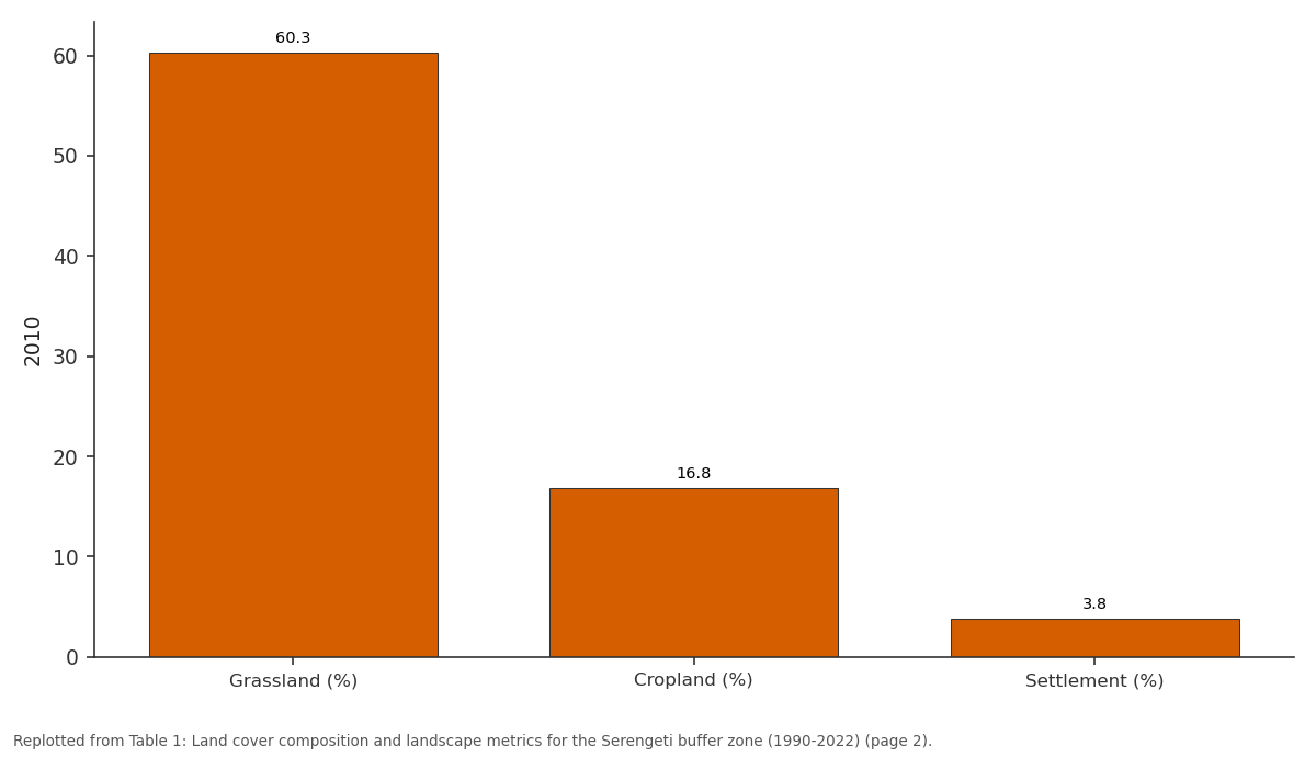
2010: Grassland (%) vs Cropland (%) vs Settlement (%)
Replotted from Table 1 (page 2) of the original paper. Every bar is the paper's own table value.
View source evidence ↗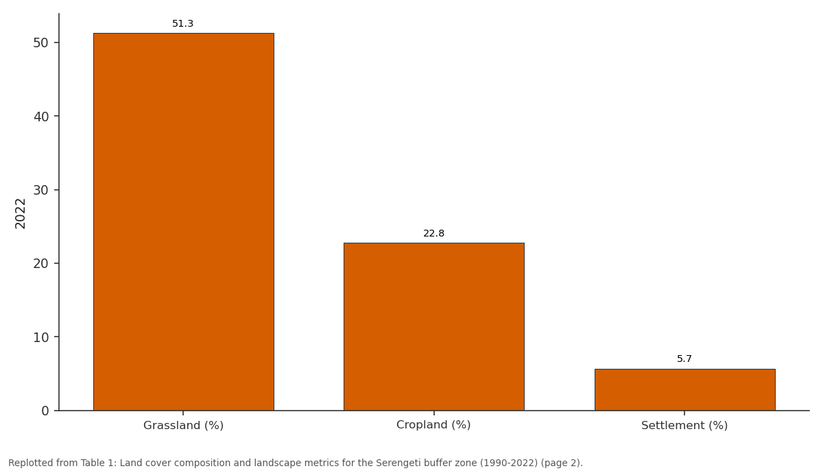
2022: Grassland (%) vs Cropland (%) vs Settlement (%)
Replotted from Table 1 (page 2) of the original paper. Every bar is the paper's own table value.
View source evidence ↗Figures & tables
From the original paper Table 1
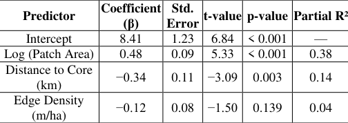 Table 2
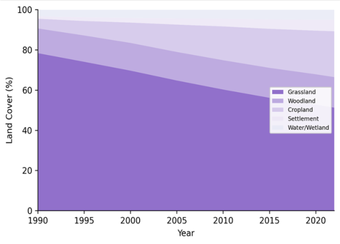 Figure 1
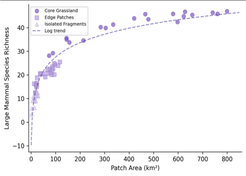 Figure 2
Introduction
Between 1990 and 2020, the human population surrounding Serengeti National Park roughly tripled, and with that growth came a wave of land conversion that is quietly reshaping one of the world's most celebrated wildlife landscapes [1] . The park itself remains legally protected, but the grasslands and woodlands in its buffer zone-the unprotected communal lands that serve as seasonal foraging grounds and migration corridors for wildebeest, zebra, and gazelle-have been progressively converted to smallholder farms and permanent settlements. This creeping transformation doesn't register as dramatic deforestation events visible from space; it proceeds field by field, homestead by homestead, gradually breaking continuous grassland into smaller and more isolated fragments. Landscape fragmentation matters for wildlife because it disrupts the spatial continuity of habitat. When a continuous grassland is subdivided by cropland and fencing, the remaining patches become smaller, more edge-dominated, and harder for animals to move between [2] . For migratory species like the Serengeti wildebeest-whose annual circuit covers roughly 800 km-even partial blockage of key corridors can alter movement patterns, compress grazing pressure into smaller areas, and increase conflict with farmers [3] . The ecological consequences extend beyond megafauna: fragmentation affects seed dispersal, fire regimes, predator-prey dynamics, and nutrient cycling in ways that cascade through the entire grassland ecosystem [4] . Landscape ecology provides a well-developed toolkit for quantifying fragmentation through spatial pattern metrics: patch area, patch density, edge density, shape complexity, and connectivity indices that describe how easily organisms can move across the landscape [5] . These metrics can be computed from classified satellite imagery using software packages like FRAGSTATS, allowing researchers to track fragmentation trajectories over time and identify the landscape elements most critical for maintaining connectivity. Previous fragmentation research in the Serengeti region has focused on the western corridor and the Mara-Serengeti boundary with Kenya [6,7] . The broader buffer zone surrounding the park-particularly the eastern and southern margins where agricultural expansion has been most rapidhas received less systematic attention. This research aimed to quantify landscape fragmentation across the entire 14,200 km² buffer zone using a 32-year satellite time series, to map the current state of ecological connectivity, and to test the relationship between patch characteristics and large mammal species richness. The work was conducted through the School of Geography and Environment in Umeå, Sweden, with field biodiversity data collected in partnership with the Tanzania Wildlife Research Institute during 2022.
Materials and Methods
Materials and Methods
Materials
Land cover data were derived from Landsat 5 TM (1990, 1995, 2000, 2005), Landsat 7 ETM + (2010), and Landsat 8 OLI (2015, 2020, 2022) imagery, all acquired during the dry season (July-September) to minimise cloud cover and seasonal phenological variation [8] . Images were downloaded from the USGS EarthExplorer archive at 30-m resolution and atmospherically corrected using the FLAASH module in ENVI 5.6. The research area comprised the 14,200 km² buffer zone defined as a 25-km radius around the boundary of Serengeti National Park, excluding the park interior. Large mammal presence data were collected between June and November 2022 at 63 sample patches selected by stratified random sampling across three fragmentation classes: core grassland (>50 km², n = 20), edge patches (10-50 km², n = 23), and isolated fragments (<10 km², n = 20). At each patch, daytime strip transects (2 km × 200 m) were walked by trained observers who recorded all large mammal species detected visually [9] .
Methods
Land cover classification used a supervised maximumlikelihood algorithm with five classes: grassland, woodland, cropland, settlement, and water/wetland. Training samples (150-200 polygons per date) were digitised from highresolution Google Earth imagery and field GPS points. Landscape metrics-number of patches (NP), mean patch area (MPA), patch density (PD), edge density (ED), and the landscape connectivity index (LCI)-were computed in FRAGSTATS 4.2 for each date using the eight-cell neighbour rule [10] . LCI was calculated as the probability that two randomly placed points in the landscape fall within the same grassland patch, ranging from 0 (completely fragmented) to 1 (single continuous patch). Species richness per patch was modelled against patch area, distance to the nearest core grassland, and edge density using multiple linear regression in R 4.2.3. Species-area relationships were fitted as log-linear models: S = c × A^z, where S is species count, A is area, and c and z are fitted constants [11] .
Field Experimental Design
The biodiversity sampling design followed a stratified random approach to ensure balanced representation across the fragmentation gradient. The 63 sample patches were assigned to three strata based on area thresholds derived from the 2022 land cover classification: core grassland patches (>50 km², retaining >80% interior habitat), edge patches (10-50 km², with high perimeter-to-area ratios), and isolated fragments (<10 km², separated from the nearest grassland patch by >2 km of non-grassland cover). Within each stratum, patches were selected randomly from the pool of all qualifying patches using the sample() function in R. Transect placement within each patch was standardised: the 2-km starting point was positioned at the patch centroid and oriented along the longest interior axis to maximise habitat coverage. All surveys were conducted between 06:30 and 10:00 local time to coincide with peak mammal activity. Observer teams consisted of one trained wildlife biologist and one local ranger familiar with the area [12] .
Calibration and Validation
Classification accuracy was assessed independently for each of the eight time steps using a stratified random sample of 250 validation points per date. Reference labels were assigned from high-resolution imagery (Google Earth for 2005-2022 dates) and from georeferenced aerial photographs archived at the Tanzania National Bureau of Statistics (for 1990-2000 dates). Overall accuracy ranged from 84.7% (1990, where reference data were less precise) to 91.3% (2022, where ground-truth data were most abundant). Kappa coefficients ranged from 0.79 to 0.88 across all dates. Grassland was the most accurately classified category (user's accuracy 89-94%), while settlement was the least accurate at earlier dates (user's accuracy 72-81%) due to its small spatial extent and spectral similarity to bare soil. Post-classification change detection was applied to identify transitions between consecutive dates, and a minimum mapping unit of 0.5 ha was imposed to reduce salt-and-pepper noise in the classified maps [13] . Figure 1 shows the scatter plot of patch area versus large mammal species richness across the 63 sampled patches.
Results
The species-area relationship was well described by the loglinear model (R² = 0.69), with core grassland patches averaging 24.7 species and isolated fragments averaging 10.8 species. Table 2 reports the multiple regression results: patch area (β = 0.48, p<0.001) and distance to nearest core grassland (β = -0.34, p<0.01) were both significant predictors of richness, together explaining 62.3% of the variance.
| Predictor | Coefficient (β) | Std. Error | t-value | p-value | Partial R² |
|---|---|---|---|---|---|
| Intercept | 8.41 | 1.23 | 6.84 | < 0.001 | — |
| Log (Patch Area) | 0.48 | 0.09 | 5.33 | < 0.001 | 0.38 |
| Distance to Core (km) | −0.34 | 0.11 | −3.09 | 0.003 | 0.14 |
| Edge Density (m/ha) | −0.12 | 0.08 | −1.50 | 0.139 | 0.04 |
Table text extracted from the original PDF; superscript letters are shown inline. The original table image is below.
View original table image
Discussion
The 27-percentage-point decline in grassland cover over 32 years translates to an annual loss rate of roughly 0.84%-a pace that, if sustained, would reduce the buffer zone's grassland to below 30% by 2050. This trajectory is alarming because landscape ecology theory suggests that connectivity collapses non-linearly once habitat cover falls below a percolation threshold, typically estimated at 40-60% depending on landscape geometry [14] . With the LCI already at 0.47 in 2022, the buffer zone may be approaching the critical threshold at which the grassland network fragments into functionally isolated patches unable to support largescale wildlife movements. The species-area relationship observed here (z = 0.31 in the log-linear model) falls within the range reported for savanna mammal assemblages in East Africa, which typically yield z-values between 0.25 and 0.35 [15] . The practical implication is clear: halving the area of a grassland patch is expected to reduce its species complement by roughly 20%. Isolated fragments smaller than 10 km² averaged only 10.8 species-fewer than half the 24.7 species found in core areas. These small patches may still serve as stepping stones for mobile species like elephants and wildebeest that can traverse cropland corridors, but they cannot sustain resident populations of less mobile species such as topi and eland, which require contiguous grassland for year-round foraging [16] .
The finding that distance to the nearest core grassland is a significant predictor of species richness (β = -0.34) reinforces the connectivity argument. Patches that are close to the park boundary or to large grassland remnants benefit from regular immigration that buffers local extinction-the "rescue effect" of metapopulation theory [17] . As agriculture fills in the gaps between patches, this rescue effect weakens, and local extinctions become permanent. Corridor planning should therefore target the narrowest constriction points where relatively small areas of land protection could maintain connectivity between the park and the remaining grassland fragments. One limitation is that the strip-transect method records only species presence, not abundance, and may underdetect cryptic or nocturnal species. Camera-trap surveys at a subset of patches would provide more complete species inventories and occupancy estimates. Additionally, the 30-m Landsat resolution may classify narrow linear corridors (<30 m wide) as non-grassland, potentially underestimating functional connectivity for species that can traverse thin habitat strips.
Conclusion
This research documented a 32-year fragmentation trajectory in the Serengeti's buffer zone, showing that grassland cover declined from 78.4% to 51.3% between 1990 and 2022. This decline was driven overwhelmingly by smallholder agricultural expansion, which converted nearly a quarter of the buffer zone to cropland. Landscape metrics confirmed the expected pattern: as grassland area shrank, patches became smaller, more numerous, and less connected, with the landscape connectivity index dropping from 0.82 to 0.47. The ecological consequences of this fragmentation are already visible. Large mammal species richness was strongly linked to patch area and proximity to core grassland, with isolated fragments smaller than 10 km² supporting fewer than half the species found in continuous habitat. The species-area and distance-richness relationships documented here provide quantitative benchmarks for predicting how further fragmentation would affect the wildlife community. These findings carry urgent implications for conservation planning in the Serengeti ecosystem. The buffer zone is not a static backdrop-it is an active participant in the ecological processes that sustain the park's globally significant wildlife populations. Protecting key corridor segments between the park and its outlying grassland patches, particularly along the eastern and southern margins where fragmentation has been fastest, should be a priority for Tanzania's wildlife management authorities. Future research should incorporate movement telemetry data from collared animals to identify the specific corridors most heavily used by migratory species and to evaluate whether existing community wildlife management areas are effectively maintaining connectivity [18] .
Acknowledgement
Acknowledgements Funding SourcesThis research was supported by general institutional research funds from the School of Geography and Environment, Umeå. No external competitive grants were applied. Institutional SupportThe authors thank the School of Geography and Environment for GIS laboratory and computing access. Field biodiversity surveys were facilitated by the Tanzania Wildlife Research Institute (TAWIRI).
Figures and tables from the paper
| Year | Grassland (%) | Cropland (%) | Settlement (%) | MPA (km²) | PD (/1000 ha) | ED (m/ha) | LCI |
|---|---|---|---|---|---|---|---|
| 1990 | 78.4 | 4.8 | 1.2 | 124.7 | 2.1 | 18.4 | 0.82 |
| 2000 | 69.7 | 10.1 | 2.4 | 87.3 | 3.2 | 27.6 | 0.71 |
| 2010 | 60.3 | 16.8 | 3.8 | 58.1 | 4.4 | 38.9 | 0.58 |
| 2022 | 51.3 | 22.8 | 5.7 | 38.4 | 5.8 | 49.3 | 0.47 |
Table text extracted from the original PDF; superscript letters are shown inline. The original table image is below.
View original table image
References
15 in the original paper- Estes AB, Kuemmerle T, Kushnir H, Radeloff VC, Shugart HH. Land-cover change and human population trends in the greater Serengeti ecosystem from 1984 to 2003. Biological Conservation. 2012;147(1):255-263.
- Fahrig L. Effects of habitat fragmentation on biodiversity. Annual Review of Ecology, Evolution, and Systematics. 2003;34(1):487-515.
- Holdo RM, Fryxell JM, Sinclair ARE, Dobson AP, Holt RD. Predicted impact of barriers to migration on the Serengeti wildebeest population. PLoS ONE. 2011;6(1):e16370.
- Haddad NM, Brudvig LA, Clobert J, Davies KF, Gonzalez A, Holt RD. Habitat fragmentation and its lasting impact on Earth's ecosystems. Science Advances. 2015;1(2):e1500052.
- McGarigal K, Cushman SA, Ene E. FRAGSTATS v4: Spatial pattern analysis program for categorical and continuous maps. University of Massachusetts. 2012;1:1-182.
- Mfunda IM, Røskaft E. Bushmeat hunting in Serengeti, Tanzania: An important economic activity to local people. International Journal of Biodiversity and Conservation. 2010;2(9):263-272.
- Ogutu JO, Owen-Smith N, Piepho HP, Said MY. Continuing wildlife population declines and range contraction in the Mara region of Kenya during 19772009. Journal of Zoology. 2011;285(2):99-109.
- Woodcock CE, Allen R, Anderson M, Belward A, Bindschadler R, Cohen W. Free access to Landsat imagery. Science. 2008;320(5879):1011.
- Buckland ST, Anderson DR, Burnham KP, Laake JL, Borchers DL, Thomas L. Introduction to distance sampling. Oxford University Press. 2001;1:1-432.
- McGarigal K, Marks BJ. FRAGSTATS: Spatial pattern analysis program for quantifying landscape structure. USDA Forest Service General Technical Report PNWGTR-351. 1995;1:1-122.
- Rosenzweig ML. Species diversity in space and time. Cambridge University Press. 1995;1:1-436.
- Sinclair ARE, Mduma SAR, Brashares JS. Patterns of predation in a diverse predator-prey system. Nature. 2003;425(6955):288-290.
- Congalton RG, Green K. Assessing the accuracy of remotely sensed data: Principles and practices. CRC Press, 2nd Edition. 2009;1:1-183.
- With KA, King AW. Extinction thresholds for species in fractal landscapes. Conservation Biology. 1999;13(2):314-326.
- Newmark WD. Insularization of Tanzanian parks and the local extinction of large mammals. Conservation Biology. 1996;10(6):1549-1556.