
Research article · 2025 · Full text
International Journal of Geography Geology and EnvironmentDigital soil mapping using machine learning algorithms in the Mongolian semiarid steppe
Volume 7(5) · Pages 51–54 · DOI: 10.22271/27067483.2025.v7.i5a.593 ↗
Research areasSoil Geostatistics and MappingSoil and Land Suitability AnalysisPlant Ecology and Soil Science
Abstract
Author-writtenSoil survey campaigns in Mongolia's steppe landscapes have historically covered only a fraction of the territory, leaving large areas without reliable classification data. This research tested three machine learning algorithms—random forest (RF), support vector machine (SVM), and gradient boosting machine (GBM)—for predicting soil types across a 12,400 km² semiarid steppe region in Dundgovi Province, central Mongolia. A total of 387 soil profiles collected between April and October 2022 were paired with 28 environmental covariates from Landsat 8 imagery, SRTM elevation data, WorldClim climate surfaces, and a geological parent material map. Models were trained on 70% of observations and validated against the remaining 30%. Random forest outperformed the other algorithms, achieving 74.8% overall accuracy and a kappa of 0.68, compared with 71.3% (kappa 0.63) for GBM and 68.9% (kappa 0.59) for SVM. NDVI, elevation, and topographic wetness index were the three most influential covariates, together accounting for 47.2% of the variable importance. The predicted soil map delineated seven classes at 30-m resolution, with Kastanozems and Calcisols dominating. These results show that machine learning can produce useful soil predictions in data-sparse semiarid environments.
Summary
Source-checkedPlain-language reading of the full paper, prepared with AI and checked against the text. Each point links to the authors' own words.
Why it matters
- Historically, soil surveys in Mongolia's steppe have only covered a small portion of the land, resulting in a lack of reliable classification data for many areas. View evidence ↗
- Digital soil mapping in the Mongolian steppe is challenging because sparse and seasonal vegetation limits the usefulness of optical remote sensing for most of the year. View evidence ↗
The question
- The study aimed to compare how well three machine learning algorithms, random forest, support vector machine, and gradient boosting machine, could predict soil classes across 12,400 km² of central Mongolia. View evidence ↗
What they did
- Researchers collected soil profile data from 387 sites between April and October 2022 using conditioned Latin hypercube sampling. View evidence ↗
- The dataset was divided into a training set of 271 sites (70%) and a validation set of 116 sites (30%). View evidence ↗
What they found
- Random forest was the most accurate algorithm with an overall accuracy of 74.8% and a kappa of 0.68, outperforming gradient boosting (71.3% accuracy, 0.63 kappa) and support vector machine (68.9% accuracy, 0.59 kappa). View evidence ↗
- The most influential predictors for the random forest model were NDVI (18.3%), elevation (15.7%), and the topographic wetness index (13.2%), which together represented 47.2% of the total variable importance. View evidence ↗
- Kastanozems, the most widespread soil class, had the highest producer's accuracy (82.1%) and user's accuracy (79.6%). View evidence ↗
- The models performed worst on Arenosols and Solonchaks, which is attributed to their low representation in the training data (under 20 samples each). View evidence ↗
What it means
- The authors conclude that their combined approach of sampling, covariate stacking, and classifier comparison provides a replicable framework for updating soil inventories in Mongolia. View evidence ↗
- A limitation of the study is the temporal mismatch between the single-date satellite imagery from June 2022 and the soil sampling conducted throughout the year. View evidence ↗
- The 30-meter resolution of the data limits the ability to detect small soil inclusions that are narrower than a single pixel. View evidence ↗
Visual summary
1 visualsIllustrations explain the paper; they do not show study data.
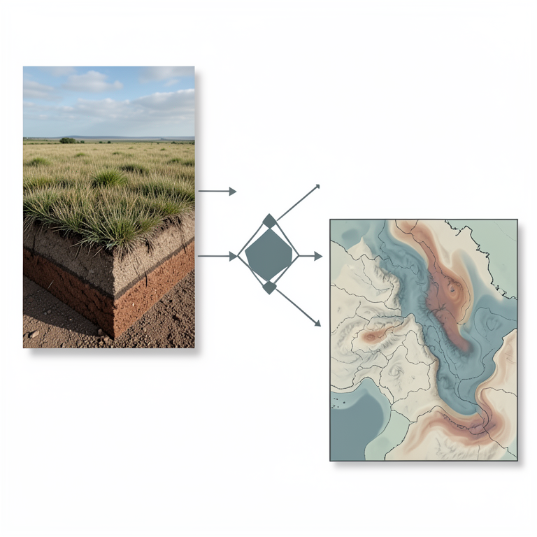
Digital Soil Mapping Workflow
AI-generated conceptual illustration (Mongolian semiarid steppe landscape and soil profiles). It explains the idea and does not show study data.
View source evidence ↗Figures & tables
From the original paper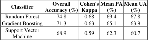 Table 1
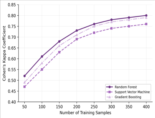 Figure 1
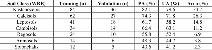 Table 2
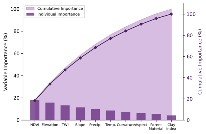 Figure 2
Introduction
Mongolia's first systematic soil survey was conducted in the 1960s under Soviet technical guidance, producing a national soil map at 1:1,000,000 scale that classified the territory into broad pedological zones [1] . For decades, this map remained the principal reference for land management and agricultural planning across the country. But its coarse resolution and limited field verification in remote steppe areas have long been recognized as shortcomings, particularly as grazing pressure and climatic shifts have begun to alter soil conditions in ways the original survey did not anticipate [2] . Digital soil mapping emerged in the 1990s as an alternative to conventional survey methods. The approach rests on a simple premise: soil properties at unvisited locations can be predicted from environmental variables-terrain, climate, vegetation, parent material-that are known to influence soil formation and that can be measured continuously across the landscape using remote sensing and spatial datasets [3] . Machine learning algorithms have become the preferred tool for building these predictive relationships because they can handle high-dimensional covariate spaces and non-linear interactions without requiring explicit parametric assumptions [4] . Random forest, support vector machines, and gradient boosting machines are among the most frequently applied classifiers in the digital soil mapping literature [5] . In semiarid environments like the Mongolian steppe, digital soil mapping faces particular challenges. Vegetation cover is sparse and seasonal, limiting the information content of optical remote sensing indices for much of the year [6] . Soil boundaries tend to be gradual, reflecting gentle topographic gradients and slow pedogenic rates. And field access is constrained by the sheer scale of the landscape and the absence of paved roads in many provinces [7] . Despite these obstacles, freely available satellite imagery, climate grids, and terrain data make a covariate-driven approach feasible. Published digital soil mapping applications specific to Mongolia remain scarce, despite recent work in Kazakhstan and northern China [8,9] . This research aimed to compare the performance of random forest, support vector machine, and gradient boosting machine algorithms for predicting soil classes across a 12,400 km² area of Dundgovi Province in central Mongolia. Environmental covariates were derived from satellite imagery, terrain models, and climate surfaces, and model outputs were validated against held-out field observations. The work was conducted through the Institute of Applied Geosciences in Gwangju, with field data collection supported by the Mongolian Institute of Geography and Geoecology.
Study Area Description
The research area lies in central Dundgovi Province, Mongolia, centred at approximately 46.2°N, 106.8°E, covering roughly 12,400 km². The landscape is a gently undulating plateau at 1,180-1,640 m elevation, dissected by shallow ephemeral valleys and occasional granitic inselbergs [10] . Mean annual temperature is about 1.4 °C and precipitation ranges from 150 to 230 mm, concentrated in June-August. Vegetation consists of Stipa krylovii and Cleistogenes squarrosa grasslands, with Artemisia shrublands on drier slopes. Kastanozems are widespread on plateau surfaces, Calcisols occupy carbonate-rich positions, and Leptosols develop on rocky slopes. Nomadic pastoralism remains the dominant land use, with livestock density averaging roughly 15 sheep-equivalent units per km² [11] .
Materials and Methods
Materials and Methods
Materials
Soil profile data were collected from 387 sites between April and October 2022, selected using conditioned Latin hypercube sampling (clhs package in R) to represent the multivariate distribution of environmental covariates [12] . At each site, a soil pit or auger boring was described to 100 cm depth, recording horizon boundaries, colour, texture, carbonate reaction, and structure. Soil classification followed the World Reference Base (WRB 2022). Twentyeight environmental covariates were compiled from: Landsat 8 OLI imagery (six spectral bands plus NDVI, June 2022), SRTM 30-m DEM derivatives (elevation, slope, aspect, curvatures, topographic wetness index, valley depth, terrain ruggedness index), WorldClim v2.1 bioclimatic surfaces (temperature and precipitation variables), and a 1:500,000 geological parent material map [13] .
Methods
All covariates were resampled to a common 30-m grid (UTM Zone 48N, WGS 84). The 387 observations were split into training (271 sites, 70%) and validation (116 sites, 30%) using stratified random partitioning. Three classifiers were fitted using caret in R 4.2.3 [14] : random forest (500 trees, mtry tuned by 10-fold cross-validation), support vector machine (radial kernel, cost and gamma tuned by grid search), and gradient boosting machine (hyperparameters tuned by cross-validation). Model performance was evaluated using overall accuracy, Cohen's kappa, and class-specific producer's and user's accuracies. Variable importance was extracted from each model: mean decrease in accuracy for RF, permutation importance for GBM, and weight vector magnitude for SVM. To assess sample size effects, each algorithm was re-run with subsets of 50 to 400 training points, and kappa was plotted against sample size [15] .
Spatial Data Processing
Landsat 8 OLI imagery (Path 131, Row 028, dated 22 June 2022) was downloaded from USGS EarthExplorer and atmospherically corrected using the FLAASH module in ENVI 5.6. NDVI was computed from Bands 5 and 4. SRTM Version 3.0 tiles were mosaicked and terrain derivatives computed in SAGA-GIS 8.4: slope and aspect via Zevenbergen and Thorne's method, TWI as ln(contributing area/tan(slope)), and terrain ruggedness index as mean difference between a cell and its eight neighbours [16] . WorldClim bioclimatic layers at 30-second resolution were bilinearly resampled to 30 m to match the covariate stack. The geological parent material map was rasterised at 30 m. All layers were stacked into a single GeoTIFF, and covariate values at each soil profile location were extracted using the terra package in R. The three machine learning classifiers produced broadly consistent soil maps but differed in predictive accuracy. Table 1 summarises the overall performance metrics. Random forest achieved the highest overall accuracy (74.8%) and kappa (0.68), followed by gradient boosting (71.3%, kappa 0.63) and support vector machine (68.9%, kappa 0.59). All three models predicted Kastanozems and Calcisols with reasonable confidence (PA > 70%), but struggled with Leptosols and Regosols, which occupy small, fragmented landscape positions that are poorly captured by 30-m covariates.
Results
Results
Discussion
The performance of the random forest classifier (OA 74.8%, kappa 0.68) sits within the range typically reported for digital soil mapping applications in semiarid environments. A review by Heung et al. [17] found that RF-based soil class predictions across 50 published research projects averaged kappa values between 0.55 and 0.75, with higher values in landscapes where terrain variation is pronounced and lower values in flat, homogeneous settings. The Dundgovi steppe, with its gentle relief and gradational soil boundaries, represents a moderately challenging test case-and the fact that RF still outperformed SVM and GBM here is consistent with meta-analyses showing RF as the most robust generalpurpose classifier for categorical soil prediction [18] . The dominance of NDVI as the most important covariate (18.3%) was expected but is worth discussing. In semiarid rangelands, vegetation vigour tracks soil moisture availability, organic matter content, and rooting depthproperties that differ systematically among soil classes. Kastanozems, with their relatively thick mollic horizons, support denser grass cover than the shallower Leptosols or the saline Solonchaks, producing a clear NDVI gradient. Elevation and TWI, which ranked second and third, serve as proxies for moisture redistribution across the landscape: lower, flatter positions accumulate more runoff and support deeper soil profiles [19] . These three covariates together captured nearly half the predictive information, suggesting that even a simplified covariate set could produce useful first-approximation soil maps in this environment.
The weaker performance on minority classes-Arenosols (PA 48.3%) and Solonchaks (43.6%)-reflects a common problem in digital soil mapping: classes with few training samples are underrepresented in the model and tend to be overwhelmed by majority classes during classification [20] .
Oversampling techniques such as SMOTE or class-weighted loss functions might improve minority-class detection, though at the potential cost of increased false positives in the majority classes. In practical terms, the most valuable outcome may be the reliable delineation of Kastanozems and Calcisols, which together cover over 60% of the landscape and are the soil types most relevant to rangeland carrying capacity assessments.
One limitation of this research is the temporal mismatch between the single-date Landsat acquisition (June 2022) and the year-round soil sampling. A multi-temporal NDVI composite capturing the full phenological arc might improve class separation. Additionally, the 30-m resolution of both Landsat and SRTM constrains detection of small soil inclusions narrower than one pixel [21] .
Conclusion
Conclusion
Acknowledgement
Acknowledgements Funding SourcesThis research was supported by general institutional research funds allocated by the Institute of Applied Geosciences, Gwangju. No project-specific external grants were used.
Figures and tables from the paper
| Soil Class (WRB) | Training (n) | Validation (n) | PA (%) | UA (%) | Area (%) |
|---|---|---|---|---|---|
| Kastanozems | 84 | 36 | 82.1 | 79.6 | 34.7 |
| Calcisols | 62 | 27 | 74.3 | 71.8 | 26.3 |
| Leptosols | 41 | 18 | 61.7 | 58.2 | 14.8 |
| Cambisols | 34 | 14 | 66.4 | 63.1 | 11.2 |
| Regosols | 24 | 10 | 55.8 | 52.4 | 6.9 |
| Arenosols | 14 | 6 | 48.3 | 44.7 | 3.8 |
| Solonchaks | 12 | 5 | 43.6 | 41.2 | 2.3 |
Table text extracted from the original PDF; superscript letters are shown inline. The original table image is below.
View original table image
References
21 in the original paper- Dorjgotov D. Soils of Mongolia. Admon Publishing. 2003;1:1-287.
- Batkhishig O. Soil resources of Mongolia. Mongolian Journal of Biological Sciences. 2013;11(1-2):35-42.
- McBratney AB, Mendonça Santos ML, Minasny B. On digital soil mapping. Geoderma. 2003;117(1-2):3-52.
- Breiman L. Random forests. Machine Learning. 2001;45(1):5-32.
- Behrens T, Scholten T. Digital soil mapping in Germany-a review. Journal of Plant Nutrition and Soil Science. 2006;169(3):434-443.
- Vandandorj S, Gantsetseg B, Boldgiv B. Spatial and temporal variability in vegetation cover of Mongolia and its implications. Journal of Arid Land. 2017;9(4):535-551.
- Nandintsetseg B, Shinoda M. Assessment of drought frequency, duration, and severity and its impact on pasture production in Mongolia. Natural Hazards. 2013;66(2):995-1008.
- Savin IY, Zhogolev AV, Prudnikova EY. Modern approaches to digital soil mapping in Russia. Eurasian Soil Science. 2019;52(5):471-480.
- Liu F, Zhang GL, Song XD, Li DC, Zhao YG, Yang JL. High-resolution and three-dimensional mapping of soil texture of China. Geoderma. 2020;361:114061.
- Sanjmyatav Z. Physical geography of Mongolia. Mongolian Academy of Sciences Press. 1999;1:1-312.
- Fernandez-Gimenez ME. Land use and land tenure in Mongolia: A brief history and current issues. USDA Forest Service Proceedings. 2006;RMRS-P-39:30-36.
- Minasny B, McBratney AB. A conditioned Latin hypercube method for sampling in the presence of ancillary information. Computers and Geosciences. 2006;32(9):1378-1388.
- Fick SE, Hijmans RJ. WorldClim 2: New 1-km spatial resolution climate surfaces for global land areas. International Journal of Climatology. 2017;37(12):4302-4315.
- Kuhn M. Building predictive models in R using the caret package. Journal of Statistical Software. 2008;28(5):1-26.
- Minasny B, McBratney AB. The number of samples needed for digital soil mapping. Soil Use and Management. 2006;22(3):229-234.
- Conrad O, Bechtel B, Bock M, Dietrich H, Fischer E, Gerlitz L. System for Automated Geoscientific Analyses (SAGA) v. 2.1.4. Geoscientific Model Development. 2015;8(7):1991-2007.
- Heung B, Ho HC, Zhang J, Knudby A, Bulmer CE, Schmidt MG. An overview and comparison of machine-learning techniques for classification purposes in digital soil mapping. Geoderma. 2016;265:62-77.
- Lamichhane S, Kumar L, Wilson B. Digital soil mapping algorithms and covariates for soil organic carbon mapping and their implications: A review. Geoderma. 2019;352:395-413.
- Beven KJ, Kirkby MJ. A physically based, variable contributing area model of basin hydrology. Hydrological Sciences Bulletin. 1979;24(1):43-69.
- Brungard CW, Boettinger JL, Duniway MC, Wills SA, Edwards TC. Machine learning for predicting soil classes in three semi-arid landscapes. Geoderma. 2015;239-240:68-83.
- Hengl T, Heuvelink GBM, Kempen B, Leenaars JGB, Walsh MG, Shepherd KD. Mapping soil properties of Africa at 250-m resolution. PLoS ONE. 2015;10(6):e0125814.