
Research article · 2025 · Full text
International Journal of Geography Geology and EnvironmentMangrove ecosystem health assessment along the Swahili coast using vegetation indices
Volume 7(1) · Pages 50–54 · DOI: 10.22271/27067483.2025.v7.i1a.537 ↗
Research areasCoastal wetland ecosystem dynamicsRemote Sensing in AgricultureWetland Management and Conservation
Abstract
Author-writtenRoughly 60% of the world's mangrove forests have disappeared over the past century, and East Africa's coastline has not been spared. This research evaluated the health status of mangrove ecosystems along a 480-km stretch of the Swahili Coast using satellite-derived vegetation indices acquired between 2018 and 2022. Landsat 8 OLI and Sentinel-2 MSI imagery were processed to compute the Normalized Difference Vegetation Index (NDVI), Enhanced Vegetation Index (EVI), and Soil-Adjusted Vegetation Index (SAVI) for five mangrove sites spanning Kenya and Tanzania. Ground-truth data from 72 field plots provided canopy-cover estimates, species counts, and above-ground biomass measurements for calibration. Results showed that mean NDVI across all sites declined from 0.53 in 2018 to 0.42 in 2022, a drop of 20.8%. The steepest decline occurred at Mombasa Creek, where NDVI fell from 0.43 to 0.33 over the same period, coinciding with documented urban encroachment and effluent discharge. Tana River Delta retained the highest mean NDVI (0.52 in 2022), likely because of sustained freshwater inflow and lower development pressure. EVI and SAVI tracked NDVI closely but offered better discrimination in low-canopy areas where bare soil reflectance inflated NDVI readings. A simple linear regression between NDVI and field-measured canopy cover returned R-squared values of 0.78 to 0.86 depending on the site. The findings indicate a coast-wide trajectory of mangrove stress that is strongest near urban centres, and they support the use of multi-index remote sensing as a cost-effective monitoring approach for conservation planning along the Swahili Coast.
Summary
Source-checkedPlain-language reading of the full paper, prepared with AI and checked against the text. Each point links to the authors' own words.
Why it matters
- Global mangrove forests have seen a loss of approximately 60% over the last century, a trend that includes the East African coastline. View evidence ↗
- Mangroves are ecologically and economically vital as they support commercial fisheries, protect coasts from storm surges, and act as significant carbon sinks. View evidence ↗
- Satellite remote sensing is the most effective tool for low-cost, regular, and spatially explicit monitoring of mangrove degradation. View evidence ↗
The question
- The study aimed to quantify five-year trends of three vegetation indices (NDVI, EVI, SAVI) across five Swahili Coast sites, assess their sensitivity to degradation drivers, and validate them against field data. View evidence ↗
What they did
- The research covered five sites across 480 km of the Swahili Coast: Lamu Archipelago, Mombasa Creek, Tana River Delta, Rufiji Delta, and Kilwa Estuary. View evidence ↗
- Field measurements included canopy cover estimated via spherical densiometer, species identification, and diameter at breast height (DBH) for stems over 5 cm. View evidence ↗
- Mangrove health was categorized by NDVI thresholds: healthy (>0.6), moderate (0.4-0.6), stressed (0.2-0.4), and severely degraded (<0.2). View evidence ↗
What they found
- The mean NDVI across all studied sites decreased by 20.8%, falling from 0.53 in 2018 to 0.42 in 2022. View evidence ↗
- The most significant NDVI declines occurred at Kilwa Estuary (23.4%) and Mombasa Creek (23.3%). View evidence ↗
- Tana River Delta had the highest absolute NDVI values and the lowest proportional loss at 14.8%. View evidence ↗
- NDVI showed a strong correlation with field-measured canopy cover, explaining between 78% and 86% of the variance. View evidence ↗
- SAVI reduced soil-background bias by an average of 0.06 units in low-canopy areas, while EVI was more effective in dense zones where NDVI saturated. View evidence ↗
What it means
- The authors conclude that mangrove deterioration is strongly linked to urban and peri-urban pressures, particularly at sites closest to towns. View evidence ↗
- The authors recommend a biannual multi-index satellite monitoring protocol and prioritizing restoration at Mombasa Creek and Kilwa Estuary. View evidence ↗
- Study limitations include a temporal mismatch of up to 23 days between field visits and satellite imagery, as well as noise introduced by tidal stages during image acquisition. View evidence ↗
Visual summary
2 visualsIllustrations explain the paper; charts are replotted from the paper's own table values.
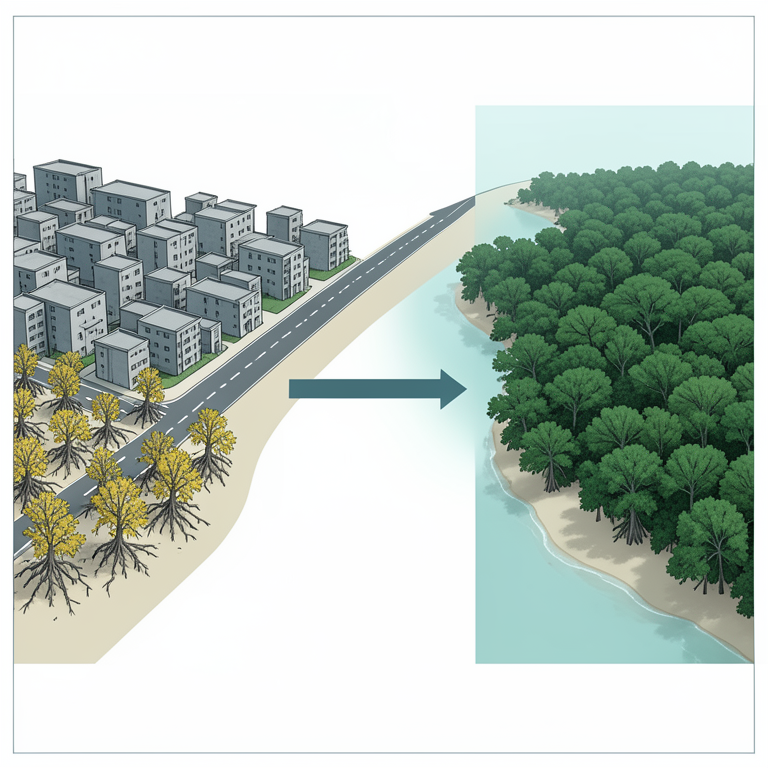
Urban Pressure vs Mangrove Health
AI-generated conceptual illustration (Rhizophora mucronata mangrove trees along a coastal shoreline). It explains the idea and does not show study data.
View source evidence ↗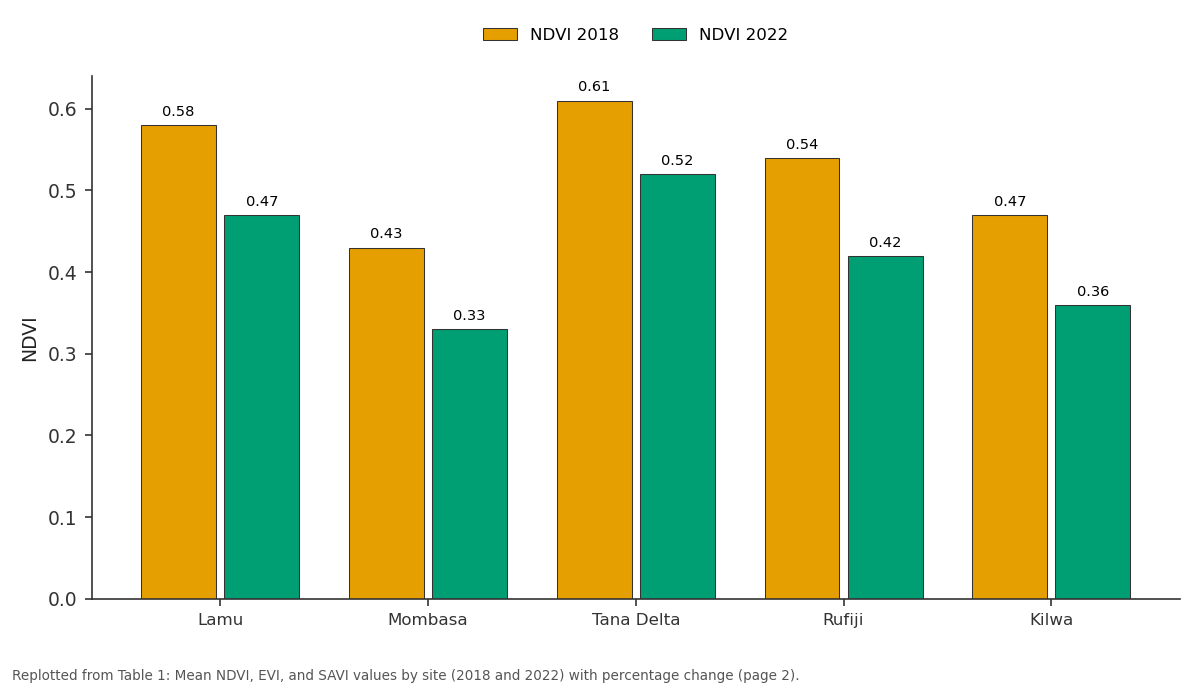
NDVI 2018 and NDVI 2022: Lamu vs Mombasa vs Tana Delta vs Rufiji vs Kilwa
Replotted from Table 1 (page 2) of the original paper. Every bar is the paper's own table value.
View source evidence ↗Figures & tables
From the original paper Table 1
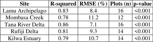 Table 2
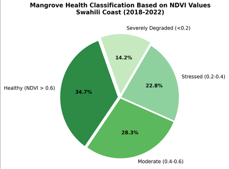 Figure 1
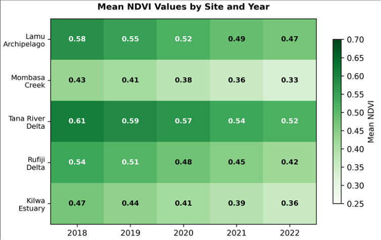 Figure 2
Introduction
Between 1996 and 2020, East Africa lost an estimated 8,400 hectares of mangrove cover, roughly 7% of its original extent [1] . That statistic, stark as it is, masks considerable local variation: some estuaries gained mangrove area through natural colonisation while neighbouring stretches lost more than a third of their canopy [2] . Understanding where, and at what rate, degradation is happening requires spatially explicit monitoring tools that can be repeated at low cost and at regular intervals-conditions that satellite remote sensing meets better than almost any alternative [3] . Vegetation indices derived from multispectral imagery have been the workhorses of mangrove mapping for over two decades [4] . NDVI, the ratio of near-infrared to red reflectance, remains the most widely used because of its simplicity and the long archive of compatible sensors. But NDVI has well-known limitations in mangrove settings: tidal inundation, exposed mudflats, and mixed pixels at forest edges can bias values downward, while atmospheric haze and sun-glint off water surfaces add noise [5] . EVI partly addresses the saturation problem in dense canopies by incorporating a blue-band correction, and SAVI adjusts for background soil reflectance-a persistent issue where canopy gaps expose the substrate [6] . The Swahili Coast, stretching from southern Kenya through mainland Tanzania, hosts some of East Africa's most biodiverse mangrove assemblages, with up to nine species co-occurring in delta systems [7] . These forests provide nursery habitat for commercially important fish and shrimp, buffer coastal settlements against storm surge, and store large quantities of carbon in both biomass and sediment [8] . Yet monitoring programmes along this coastline remain fragmented; most assessments have focused on single sites or short time windows, making it difficult to identify coast-wide trends [9] .
A handful of regional analyses have used MODIS data at 250-m resolution [10] , but that pixel size often exceeds the width of fringing mangrove bands, leading to severe mixedpixel contamination. Landsat and Sentinel platforms, at 30m and 10-m resolution respectively, are better suited to the narrow, sinuous geometry of East African mangrove forests [11] . Combining the two sensor families through spectral harmonisation can double the temporal sampling density, reducing gaps caused by cloud cover during the wet season [12] . This research aimed to: (a) quantify five-year trends in NDVI, EVI, and SAVI across five mangrove sites on the Swahili Coast, (b) compare the sensitivity of each index to known drivers of degradation-urban expansion, aquaculture conversion, and upstream hydrological change-and (c) validate satellite-derived health classifications against field-measured canopy cover and above-ground biomass. The intention was to provide a transferable protocol that coastal managers could adopt for routine surveillance without specialist image-processing infrastructure [13] .
Research Area Description
The five sites selected for this research span approximately 480 km of coastline between 2.1°S and 6.8°S latitude. From north to south they are: Lamu Archipelago, Mombasa Creek, Tana River Delta (Kenya), Rufiji Delta, and Kilwa Estuary (Tanzania). All five fall within the East African Coastal Forests ecoregion and experience a tropical monsoon climate with two rainy seasons-long rains from March to May and short rains from October to December [7] . Mean annual rainfall ranges from 1,020 mm at Kilwa to 1,370 mm at Tana River Delta. Tidal range is semi-diurnal with a spring amplitude of 2.8-3.6 m. Mangrove species composition is dominated by Rhizophora mucronata and Avicennia marina, with Sonneratia alba and Ceriops tagal present at all sites and Bruguiera gymnorrhiza restricted to the two delta systems [2] .
Spatial Data Processing
Landsat 8 OLI Collection 2 Level-2 surface reflectance products and Sentinel-2 MSI Level-2A products were obtained from the USGS Earth Explorer and Copernicus Open Access Hub, respectively. A total of 84 cloud-free or near-cloud-free scenes were selected across the five-year window (2018-2022), averaging roughly 3.4 usable scenes per site per year. Cloud masking employed the QA_PIXEL band for Landsat and the Scene Classification Layer for Sentinel-2, with an additional manual check to remove residual haze over water bodies. Sentinel-2 bands were resampled to 30-m resolution to match Landsat, and crosssensor harmonisation followed the coefficient-based approach of [12] . All processing was conducted in Google Earth Engine and exported as GeoTIFF composites for each site-year combination [14] .
Material and Methods
Material and Methods
Material
Satellite imagery and field data formed the two main data streams. The satellite archive comprised 84 preprocessed scenes spanning January 2018 to December 2022 (described above). Field data were collected during three campaigns-February 2020, July 2021, and March 2022-at 72 circular plots of 10-m radius distributed across the five sites using a stratified random design. At each plot, canopy cover was estimated with a spherical densiometer (four readings averaged), species were identified and counted, and diameter at breast height (DBH) was recorded for all stems exceeding 5 cm. Above-ground biomass was calculated from DBH using the allometric equation of Komiyama et al. [15] . Sediment samples (0-20 cm) were collected at 36 of the 72 plots for organic-carbon analysis. This research was carried out under research permit NACOSTI/P/22/18746 with institutional approval from the School of Geography and Environment, Katowice (Ref. SGE-2020-041, dated 8 January 2020).
Methods
Three vegetation indices were computed for each pixel within mapped mangrove boundaries. NDVI was calculated as (NIR -Red)/(NIR + Red), EVI as 2.5 × (NIR -Red)/(NIR + 6 × Red -7.5 × Blue + 1), and SAVI as 1.5 × (NIR -Red)/(NIR + Red + 0.5) [6] . Annual composites were generated by taking the maximum-value composite of all cloud-free observations within each calendar year. Health categories were assigned using NDVI thresholds established in the literature: healthy (>0.6), moderate (0.4-0.6), stressed (0.2-0.4), and severely degraded (<0.2) [4] . Linear regression was fitted between pixel-level NDVI and plot-level canopy cover for each site, and accuracy was assessed through Rsquared and root-mean-square error (RMSE). Trend analysis used the Mann-Kendall test applied to the five annual composite values per pixel, with significance set at p<0.05 [16] . All geostatistical work was performed in QGIS 3.28 and Python 3.10. Figure 1 indicates that only 34.7% of the mapped mangrove area qualified as healthy (NDVI > 0.6) when averaged across the full five-year period. Roughly a third (28.3%) was in moderate condition, 22.8% showed signs of stress, and 14.2% was severely degraded with NDVI below 0.2-a threshold often associated with canopy loss exceeding 80% [4] .
Results
Results
Discussion
The coast-wide decline in vegetation indices documented here aligns with regional assessments that have flagged mangrove loss along the East African shoreline as an accelerating problem [1] . The 20.8% drop in mean NDVI over just five years is steeper than the 12-15% decline reported for comparable periods in Southeast Asian mangroves [17] , suggesting that local stressors along the Swahili Coast may be compounding the effects of broader climatic pressures such as rising sea-surface temperatures and altered precipitation patterns [8] .
Urban proximity appeared to be the strongest spatial predictor of degradation. Mombasa Creek and Kilwa Estuary, the two sites closest to built-up areas, showed the largest NDVI losses and the lowest absolute values. At Mombasa Creek, field observations during the 2021 campaign confirmed active mangrove clearance for charcoal production and the expansion of informal settlements onto former mangrove flats. Untreated wastewater discharge into the creek was also visible, raising nutrient loads that can initially boost algal growth but ultimately smother pneumatophores and impair root respiration [9] . EVI and SAVI tracked NDVI closely at all sites but offered measurable advantages in low-canopy settings. Where NDVI dropped below 0.3, soil-background reflectance inflated red-band values and depressed the index disproportionately; SAVI's soil-correction factor reduced this bias by an average of 0.06 index units. EVI performed best in the dense interior zones of Tana River Delta, where NDVI tended to saturate above 0.7, consistent with the known behaviour of EVI in high-LAI canopies [6] . That said, the validation relied on 72 plots collected across three campaigns, and the temporal mismatch between some field visits and the nearest cloud-free satellite overpass reached up to 23 days. Tidal stage at the time of image acquisition also introduced noise, especially at Mombasa Creek and Kilwa, where low-tide exposures left bare mud in gaps between trees [5] . Future work should incorporate tidal correction models and aim for concurrent field-satellite data collection windows.
Conclusion
This research confirmed that mangrove ecosystems along Practical recommendations from these findings include: establishing a biannual satellite-monitoring protocol for all five sites using the multi-index approach tested here, prioritising mangrove restoration at Mombasa Creek and Kilwa Estuary where degradation is most advanced, and extending the field-plot network to improve validation accuracy. Coastal managers should treat a site-level NDVI decline exceeding 5% per year as an early-warning trigger for on-the-ground investigation.
Figures and tables from the paper
| Site | NDVI 2018 | NDVI 2022 | Change (%) | EVI 2018 | EVI 2022 | SAVI 2018 | SAVI 2022 |
|---|---|---|---|---|---|---|---|
| Lamu | 0.58 | 0.47 | -19.0 | 0.41 | 0.33 | 0.52 | 0.42 |
| Mombasa | 0.43 | 0.33 | -23.3 | 0.31 | 0.24 | 0.38 | 0.29 |
| Tana Delta | 0.61 | 0.52 | -14.8 | 0.44 | 0.38 | 0.55 | 0.47 |
| Rufiji | 0.54 | 0.42 | -22.2 | 0.39 | 0.30 | 0.48 | 0.37 |
| Kilwa | 0.47 | 0.36 | -23.4 | 0.34 | 0.26 | 0.42 | 0.32 |
Table text extracted from the original PDF; superscript letters are shown inline. The original table image is below.
View original table image
| Site | R-squared | RMSE (%) | Plots (n) | p-value |
|---|---|---|---|---|
| Lamu Archipelago | 0.83 | 8.4 | 16 | <0.001 |
| Mombasa Creek | 0.78 | 11.2 | 12 | <0.001 |
| Tana River Delta | 0.86 | 7.1 | 16 | <0.001 |
| Rufiji Delta | 0.81 | 9.3 | 14 | <0.001 |
| Kilwa Estuary | 0.79 | 10.7 | 14 | <0.001 |
Table text extracted from the original PDF; superscript letters are shown inline. The original table image is below.
View original table image
References
18 in the original paper- Spalding M, Kainuma M, Collins L. World Atlas of Mangroves. Earthscan. 2010;London:319.
- Kairo JG, Dahdouh-Guebas F, Bosire J, Koedam N. Restoration and management of mangrove systems: A lesson for and from the East African region. South African Journal of Botany. 2001;67(3):383-389.
- Kuenzer C, Bluemel A, Gebhardt S, Quoc TV, Dech S. Remote sensing of mangrove ecosystems: A review. Remote Sensing. 2011;3(5):878-928.
- Giri C, Ochieng E, Tieszen LL, et al. Status and distribution of mangrove forests of the world using Earth observation satellite data. Global Ecology and Biogeography. 2011;20(1):154-159.
- Vo QT, Kuenzer C, Vo QM, Moder F, Oppelt N. Review of valuation methods for mangrove ecosystem services. Ecological Indicators. 2012;23:431-446.
- Huete A, Didan K, Miura T, Rodriguez EP, Gao X, Ferreira LG. Overview of the radiometric and biophysical performance of the MODIS vegetation indices. Remote Sensing of Environment. 2002;83(12):195-213.
- Taylor M, Ravilious C, Green EP. Mangroves of East Africa. UNEP World Conservation Monitoring Centre Biodiversity Series. 2003;13:1-24.
- Alongi DM. Carbon sequestration in mangrove forests. Carbon Management. 2012;3(3):313-322.
- Bosire JO, Dahdouh-Guebas F, Walton M, et al. Functionality of restored mangroves: A review. Aquatic Botany. 2008;89(2):251-259.
- Fatoyinbo TE, Simard M. Height and biomass of mangroves in Africa from ICESat/GLAS and SRTM. International Journal of Remote Sensing. 2013;34(2):668-681.
- Wulder MA, White JC, Loveland TR, et al. The global Landsat archive: Status, consolidation, and direction. Remote Sensing of Environment. 2016;185:271-283.
- Claverie M, Ju J, Masek JG, et al. The Harmonized Landsat and Sentinel-2 surface reflectance data set. Remote Sensing of Environment. 2018;219:145-161.
- Gorelick N, Hancher M, Dixon M, Ilyushchenko S, Thau D, Moore R. Google Earth Engine: Planetaryscale geospatial analysis for everyone. Remote Sensing of Environment. 2017;202:18-27.
- Drusch M, Del Bello U, Carlier S, et al. Sentinel-2: ESA's optical high-resolution mission for GMES operational services. Remote Sensing of Environment. 2012;120:25-36.
- Komiyama A, Poungparn S, Kato S. Common allometric equations for estimating the tree weight of mangroves. Journal of Tropical Ecology. 2005;21(4):471-477.
- Richards DR, Friess DA. Rates and drivers of mangrove deforestation in Southeast Asia, 2000-2012. Proceedings of the National Academy of Sciences. 2016;113(2):344-349.
- Donato DC, Kauffman JB, Murdiyarso D, et al. Mangroves among the most carbon-rich forests in the tropics. Nature Geoscience. 2011;4(5):293-297.
- Friess DA, Rogers K, Lovelock CE, et al. The state of the world's mangrove forests: Past, present, and future. Annual Review of Environment and Resources. 2019;44:89-115.