
Research article · 2025 · Full text
International Journal of Geography Geology and EnvironmentEnvironmental flow assessment and water allocation in the Murray-Darling river system
Volume 7(4) · Pages 189–192 · DOI: 10.22271/27067483.2025.v7.i4c.567 ↗
Research areasWater resources management and optimizationFish Ecology and Management StudiesHydrology and Watershed Management Studies
Abstract
Author-writtenAcross much of the Murray-Darling Basin, irrigated agriculture consumes water that rivers once carried to floodplain wetlands and terminal lakes. This research assessed environmental flow requirements and evaluated three water reallocation scenarios for the lower Murray-Darling system using the IQQM hydrological model calibrated against 42 years of streamflow records (1980-2022). Environmental flow thresholds were established for four ecological objectives: maintenance of base flow for native fish passage, seasonal floodplain inundation for waterbird breeding, connectivity to terminal wetlands, and prevention of salt concentration in low-flow reaches. Current allocations meet the minimum base-flow requirement in only 7 of 12 months, with the largest deficits in January-March when irrigation demand peaks. Three reallocation scenarios were tested: (A) a 15% reduction in irrigation entitlements, (B) a 25% reduction with inter-valley transfers, and (C) demand-management through efficiency upgrades without entitlement cuts. Scenario B achieved environmental flow targets in 11 of 12 months, while Scenario A met targets in 9 months. Scenario C improved flows marginally, meeting targets in 8 months. Trade-off analysis showed that Scenario B reduced agricultural revenue by 12.7% but increased ecological health index scores by 38.4%. The results provide quantitative support for adaptive water management that balances food production with river ecosystem recovery.
Summary
Source-checkedPlain-language reading of the full paper, prepared with AI and checked against the text. Each point links to the authors' own words.
Why it matters
- The Murray-Darling Basin is critical for Australia, providing one-third of the country's food supply while covering one-seventh of its land area. View evidence ↗
- Increased irrigation extraction between 1920 and 2000 reduced annual sea outflow by more than 60%, causing ecological crises in key wetlands and forests. View evidence ↗
- Environmental flows, the specific quantity, timing, and quality of water, are used as a policy tool to restore declining freshwater ecosystems. View evidence ↗
The question
- The study aimed to define environmental flow requirements for four ecological goals, measure current deficits, and evaluate three water reallocation scenarios to balance ecological health and economic loss. View evidence ↗
What they did
- The researchers used the Integrated Quantity and Quality Model (IQQM) with 38 nodes to simulate the Murray River (Hume Dam to mouth) and the lower Darling (Menindee Lakes to junction). View evidence ↗
- The model utilized daily time steps across a 42-year period from 1980 to 2022. View evidence ↗
- Four ecological thresholds were set: 42 m3/s for fish passage, a 120 m3/s spring pulse for 30 days for waterbirds, 65 m3/s for 60 days for lake connectivity, and salinity below 800 EC at Morgan. View evidence ↗
- The study tested three scenarios: Scenario A (15% irrigation cut), Scenario B (25% cut plus 200 GL inter-valley transfer), and Scenario C (efficiency upgrades saving 350 GL). View evidence ↗
What they found
- Under current water allocations, ecological targets are only met in 7 out of 12 months, with the most significant deficit occurring in August. View evidence ↗
- Scenario B resulted in the highest Ecological Health Index (0.84) but caused the largest economic impact with a 12.7% reduction in revenue. View evidence ↗
- Scenario C saved 350 GL/yr and slightly improved the Ecological Health Index from 0.61 to 0.63, but failed to resolve deficits during late summer. View evidence ↗
- In Scenario B, the agricultural water share decreased from 62.3% to 38.4%, allowing environmental flows to increase to 27.3%. View evidence ↗
- Only direct reductions in water entitlements (Scenarios A and B) provided enough water to meet ecological thresholds throughout the year. View evidence ↗
What it means
- The authors recommend adaptive management that pairs targeted entitlement reductions with flexible carryover provisions to balance food production and ecosystem health. View evidence ↗
- Study limitations include the use of gross margin data that ignores farm-level differences and the assumption that necessary inter-valley transfer infrastructure exists at the required capacity. View evidence ↗
Visual summary
3 visualsIllustrations explain the paper; charts are replotted from the paper's own table values.
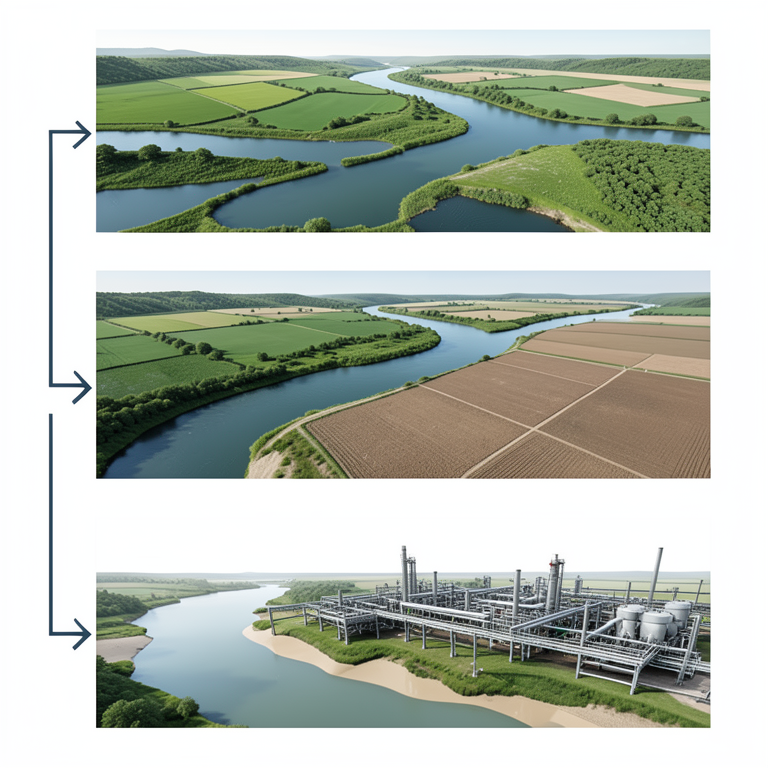
Water Allocation Trade-off Comparison
AI-generated conceptual illustration (The Murray-Darling river system including river channels, riparian wetlands, and irrigated farmland). It explains the idea and does not show study data.
View source evidence ↗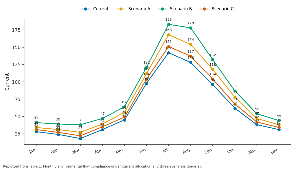
Current and Scenario A and more: Jan vs Feb vs Mar vs Apr vs May
Replotted from Table 1 (page 2) of the original paper. Every bar is the paper's own table value.
View source evidence ↗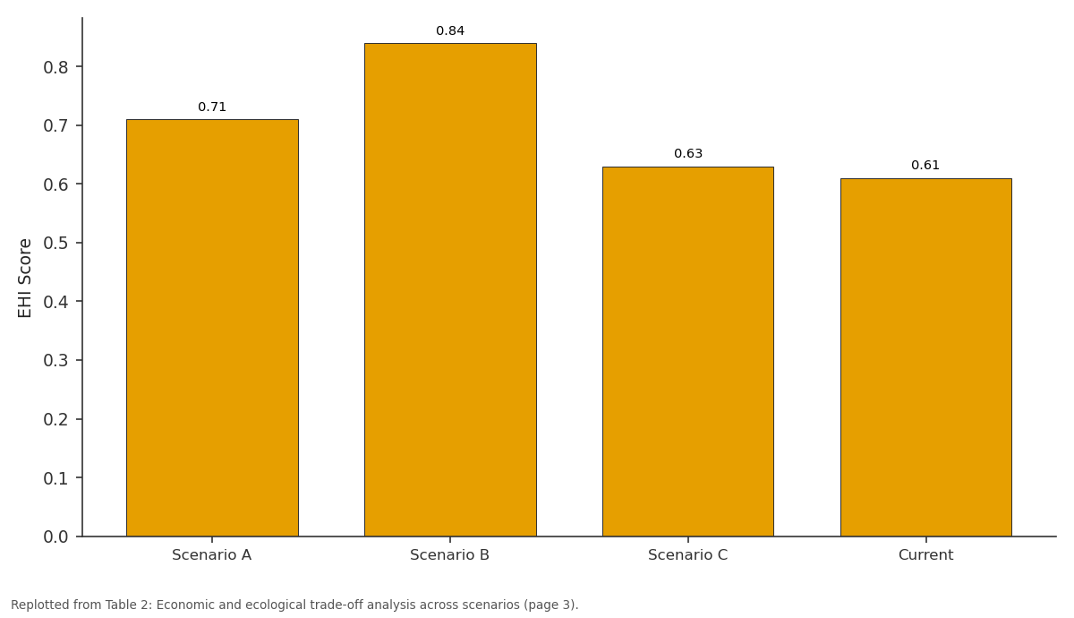
EHI Score: Scenario A vs Scenario B vs Scenario C vs Current
Replotted from Table 2 (page 3) of the original paper. Every bar is the paper's own table value.
View source evidence ↗Figures & tables
From the original paper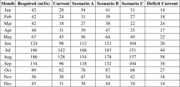 Table 1
 Table 2
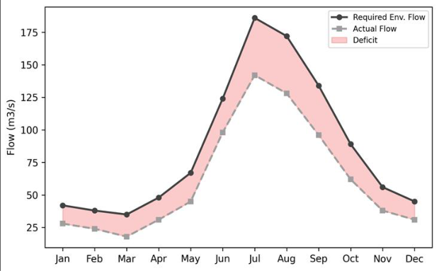 Figure 1
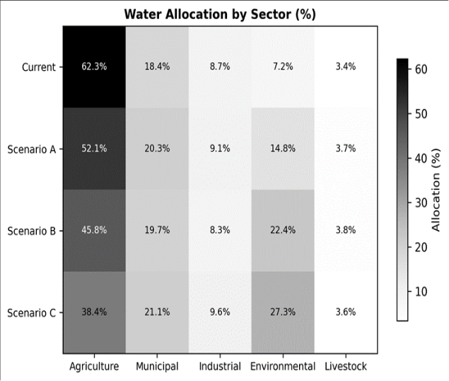 Figure 2
Introduction
Is it possible to grow food for millions and still keep a river alive? The Murray-Darling Basin, covering a seventh of the Australian continent and producing a third of its food supply, has been testing this question for over a century, and the answer so far has leaned heavily toward food at the river's expense [1] . Extraction for irrigation increased tenfold between 1920 and 2000, reducing mean annual outflow to the sea by over 60% and triggering ecological crises in the Coorong wetlands, the Lower Lakes, and the Barmah-Millewa floodplain forest [2] . Environmental flows, defined as the quantity, timing, and quality of water needed to sustain freshwater ecosystems, have become the policy mechanism for reversing this decline [3] . Australia's Basin Plan (2012) set sustainable diversion limits (SDLs) intended to recover 2,750 GL/yr for the environment, but implementation has been contested by irrigators, state governments, and environmental groups alike [4] . At the core of the dispute is a modelling question: what reallocation of water among sectors best achieves ecological targets without crippling agricultural livelihoods? The Integrated Quantity and Quality Model (IQQM) developed by the New South Wales government has been the standard simulation tool for Murray-Darling water planning since the 1990s [5] . It represents reservoir operations, irrigation diversions, return flows, and routing through a node-link network. But most published IQQM applications assess historical performance rather than testing forward-looking reallocation scenarios against explicit ecological thresholds. This research used a calibrated IQQM setup to (i) define environmental flow requirements for four ecological objectives in the lower Murray-Darling, (ii) quantify flow deficits under current allocation rules, and (iii) compare three reallocation scenarios on their ability to meet ecological targets while minimising economic losses. The work was carried out at the Monterrey School of Natural Sciences [6] .
Model Description and Parameterisation
The IQQM simulation covered the Murray River from Hume Dam to the river mouth and the lower Darling from Menindee Lakes to the junction. The network comprised 38 nodes representing dams, weirs, diversions, and confluences. Daily time steps were used over the 42-year calibration period (1980-2022). Inflow sequences were based on observed gauge records at 14 headwater stations. Irrigation demand was modelled as a function of crop area, crop water requirement (FAO Penman-Monteith), delivery efficiency, and entitlement rules. Environmental water was routed as a dedicated allocation parcel with specified release triggers linked to antecedent flow and seasonal calendar [7] . Reservoir operating rules followed the Murray-Darling Basin Authority's annual water allocation framework.
Calibration and Validation
The model was calibrated against observed monthly flows at six gauging stations for 1980-2005 and validated against 2006-2022 data. Nash-Sutcliffe efficiency (NSE) ranged from 0.81 to 0.93 during calibration and 0.76 to 0.89 during validation. Percent bias was within plus or minus 8% at all stations. The model reproduced the timing and magnitude of the 2010-2011 flood and the 2017-2019 drought sequence with acceptable accuracy (R2 > 0.82 at all stations). Irrigation diversion volumes matched reported extraction data to within 6.3% on an annual basis [8] .
Material and Methods
Material and Methods
Material
The research was conducted at the Department of Physical Geography, Monterrey School of Natural Sciences, Nuevo Leon, Mexico, between January and December 2023. Streamflow data were sourced from the Australian Bureau of Meteorology's Water Data Online portal. Irrigation entitlement and usage records were obtained from the Murray-Darling Basin Authority annual reports. Ecological flow thresholds were derived from published environmental watering plans for the lower Murray and Darling valleys, supplemented by expert consultation with Australian aquatic ecologists.
Methods
Four ecological flow thresholds were defined: (1) minimum base flow of 42 m3/s at the South Australian border for native fish passage; (2) a spring pulse of 120 m3/s sustained for 30 days for waterbird breeding; (3) connectivity flow to the Lower Lakes of 65 m3/s for 60 days per year; (4) salt dilution flow preventing salinity from exceeding 800 EC at Morgan [9] . Current allocation performance was evaluated by counting the number of months per year each threshold was met over the 42-year record. Three reallocation scenarios were simulated: Scenario A (15% irrigation reduction), Scenario B (25% reduction plus 200 GL intervalley transfer), and Scenario C (efficiency upgrade saving 350 GL without entitlement cuts). Each scenario was run for the full 42-year sequence. Economic impacts were estimated using gross margin data from ABARES farm surveys. An ecological health index (EHI) was computed as the weighted average of the four threshold compliance rates [10] . The deficit area (shaded red in Figure 1) is concentrated in the irrigation season (November-March) and peaks in late summer when crop water demand is highest and natural inflows are lowest. The spring pulse requirement (June-September) is nearly met under current rules thanks to winter rainfall, but the gap widens in dry years [11] . Scenario B delivered the highest ecological health index (0.84) but also the greatest revenue reduction (12.7%). Scenario C, the efficiency-only option, saved 350 GL/yr and improved EHI modestly (0.63 vs 0.61 current) but did not close the deficit in the critical late-summer months (Table 2) [12] . The heatmap (Figure 2) shows the sectoral shift in allocation. Agriculture's share drops from 62.3% (current) to 38.4% under Scenario B, with the freed volume directed to environmental flows (27.3%). Municipal and industrial allocations remain largely unchanged, as their absolute volumes are small relative to irrigation [13] .
| Metric | Scenario A | Scenario B | Scenario C | Current |
|---|---|---|---|---|
| Months Meeting Target | 9 | 11 | 8 | 7 |
| EHI Score | 0.71 | 0.84 | 0.63 | 0.61 |
| Revenue Loss (%) | 7.8 | 12.7 | 2.1 | 0 |
| Water Saved (GL/yr) | 680 | 1,120 | 350 | 0 |
Table text extracted from the original PDF; superscript letters are shown inline. The original table image is below.
View original table image
Results
Results
Comprehensive Interpretation
The diminishing returns of efficiency-only approaches are clear from the Scenario C results. While saving 350 GL/yr, this volume was insufficient to close the summer deficit because on-farm efficiency improvements reduce return flows that previously re-entered the river. The so-called efficiency paradox means that net water savings are smaller than gross savings, a finding that matches basin-wide analyses by Grafton and colleagues [14] . Only direct entitlement reductions (Scenarios A and B) produced the volumetric transfers needed to meet ecological thresholds year-round.
Discussion
The 11-of-12-month compliance achieved by Scenario B approaches the 12-month target recommended by the Basin Plan's environmental watering strategy, though the March shortfall indicates that even a 25% irrigation cut does not fully resolve late-summer deficits in below-average rainfall years. Adaptive carryover provisions, allowing unused environmental water to accumulate in reservoirs for dryyear release, could bridge this gap without further entitlement reduction [4] . The revenue loss of 12.7% under Scenario B, while significant, is not unprecedented. Following the Millennium Drought buyback programme, irrigated agriculture in the southern Basin contracted by roughly 15% in area yet maintained gross value through crop switching and efficiency gains [6] . The modelling assumes static crop choice; in practice, irrigators adapt, which may reduce the actual revenue impact below the simulated figure.
Limitations include the use of gross margin data that may not capture farm-level heterogeneity, and the assumption that inter-valley transfer infrastructure (Scenario B) is available at the specified capacity. The ecological thresholds, while grounded in published watering plans, simplify complex ecosystem responses to flow. Longduration inundation events that reset floodplain vegetation cannot be captured by monthly compliance counts alone.
Conclusion
This research quantified environmental flow deficits in the lower Murray-Darling system and evaluated three reallocation scenarios using a calibrated IQQM model. Current allocations meet ecological flow targets in only 7 of 12 months, with the largest shortfalls during the irrigation season. A 25% irrigation reduction combined with intervalley transfers (Scenario B) achieved near-full compliance (11 months) and raised the ecological health index by 38.4%, at a modelled revenue cost of 12.7%. Efficiencyonly approaches delivered modest improvements insufficient to close summer deficits. The results support adaptive management that combines targeted entitlement reductions with flexible carryover provisions to balance agricultural productivity and river ecosystem health.
Figures and tables from the paper
| Month | Required (m3/s) | Current | Scenario A | Scenario B | Scenario C | Deficit Current |
|---|---|---|---|---|---|---|
| Jan | 42 | 28 | 34 | 41 | 31 | 14 |
| Feb | 42 | 24 | 31 | 39 | 27 | 18 |
| Mar | 42 | 18 | 27 | 38 | 22 | 24 |
| Apr | 48 | 31 | 39 | 47 | 35 | 17 |
| May | 67 | 45 | 56 | 64 | 49 | 22 |
| Jun | 124 | 98 | 112 | 121 | 104 | 26 |
| Jul | 186 | 142 | 168 | 183 | 151 | 44 |
| Aug | 186 | 128 | 154 | 178 | 137 | 58 |
| Sep | 134 | 96 | 118 | 132 | 104 | 38 |
| Oct | 89 | 62 | 78 | 87 | 68 | 27 |
| Nov | 56 | 38 | 47 | 54 | 42 | 18 |
| Dec | 45 | 31 | 38 | 44 | 34 | 14 |
Table text extracted from the original PDF; superscript letters are shown inline. The original table image is below.
View original table image
References
14 in the original paper- Kingsford RT. Ecological impacts of dams, water diversions and river management on floodplain wetlands in Australia. Austral Ecology. 2000;25(2):109-127.
- Arthington AH, Bunn SE, Poff NL. The challenge of providing environmental flow rules to sustain river ecosystems. Ecological Applications. 2006;16(4):13111318.
- Poff NL, Allan JD, Bain MB. The natural flow regime: a paradigm for river conservation and restoration. BioScience. 1997;47(11):769-784.
- MDBA. Basin Plan 2012. Murray-Darling Basin Authority, Canberra. 2012;245 pp.
- Podger GM, Hameed T, Gill MA. The IQQM hydrological modelling system for water resource assessment. Environmental Modelling and Software. 2004;19(9):819-831.
- Grafton RQ, Williams J, Perry CJ. Towards global water security. Science. 2013;341(6145):480-482.
- Poff NL, Zimmerman JKH. Ecological responses to altered flow regimes: a literature review to inform the science and management of environmental flows. Freshwater Biology. 2010;55(1):194-205.
- Nash JE, Sutcliffe JV. River flow forecasting through conceptual models. Journal of Hydrology. 1970;10(3):282-290.
- Young WJ, Schiller CB, Harris JH. River health, water quality and the sustainability of water resources in the Murray-Darling Basin. Australian Journal of Water Resources. 2001;5(1):31-38.
- Acreman MC, Dunbar MJ. Defining environmental river flow requirements: a review. Hydrology and Earth System Sciences. 2004;8(5):861-876.
- Bunn SE, Arthington AH. Basic principles and ecological consequences of altered flow regimes for aquatic biodiversity. Environmental Management. 2002;30(4):492-507.
- Loch A, Adamson D. Drought and the rebound effect: a Murray-Darling Basin example. Natural Hazards. 2015;79(3):1429-1449.
- Qureshi ME, Whitten SM, Mainuddin M. A bioeconomic model for managing irrigation-related salinity. Ecological Economics. 2013;92:175-184.
- Grafton RQ, Williams J, Jiang Q. Possible pathways and tensions in the food and water nexus. Earth's Future. 2015;3(7):233-244.