
Research article · 2025 · Full text
International Journal of Geography Geology and EnvironmentAnalysis of landform classification using object-based image analysis in the Tibetan Plateau
Volume 7(4) · Pages 193–196 · DOI: 10.22271/27067483.2025.v7.i4c.569 ↗
Research areasRemote-Sensing Image ClassificationRemote Sensing and Land UseLandslides and related hazards
Abstract
Author-writtenMapping landforms across the Tibetan Plateau has traditionally relied on manual interpretation, a process that is subjective and difficult to replicate at regional scale. This research applied object-based image analysis (OBIA) to classify landforms across a 28,400 km2 area of the central Tibetan Plateau using a 30 m ASTER GDEM supplemented by Sentinel-2 multispectral imagery. The classification targeted six landform classes: glacial, fluvial, aeolian, structural, periglacial, and lacustrine. Image segmentation was performed in eCognition Developer 10.0 using a multi-resolution algorithm, producing 14,287 objects at the optimal scale parameter (SP = 45). A random forest classifier trained on 420 ground-truth points (70 per class) achieved an overall accuracy of 87.3% and a Kappa coefficient of 0.85. Glacial landforms covered the largest share (24.3%), followed by fluvial (19.8%) and structural (18.7%). Producer accuracy was highest for lacustrine features (93.1%) and lowest for periglacial (78.4%), reflecting spectral confusion between periglacial solifluction lobes and aeolian deposits. Variable importance analysis identified slope, plan curvature, and NDVI as the three most discriminating terrain derivatives. Comparison with a pixel-based maximum likelihood classification on the same data showed that OBIA improved overall accuracy by 8.7 percentage points, mainly by reducing salt-and-pepper noise in heterogeneous terrain. The resulting landform map serves as a baseline for geomorphological research and land-use planning on the plateau.
Summary
Source-checkedPlain-language reading of the full paper, prepared with AI and checked against the text. Each point links to the authors' own words.
Why it matters
- The Tibetan Plateau is a critical region as it contains the largest ice reservoir outside polar areas and supports nearly two billion people via its river systems. View evidence ↗
- Traditional landform mapping in this region has been limited by manual interpretation, which is subjective and hard to scale up. View evidence ↗
- Object-based image analysis (OBIA) is preferred over pixel-based methods because it uses spatial units (objects) to include shape, texture, and context. View evidence ↗
The question
- The study aimed to create an OBIA workflow for regional landform classification, compare its accuracy to pixel-based methods, and determine which terrain derivatives best distinguish between six landform classes. View evidence ↗
What they did
- The researchers analyzed a 28,400 km² area of the central Tibetan Plateau using 30 m ASTER GDEM and Sentinel-2 multispectral imagery. View evidence ↗
- The study focused on classifying six specific landform types: glacial, fluvial, aeolian, structural, periglacial, and lacustrine. View evidence ↗
- Using eCognition Developer 10.0, the team performed image segmentation with a scale parameter of 45, resulting in 14,287 objects. View evidence ↗
- A random forest classifier was trained using 420 ground-truth points, with 70 points allocated to each of the six classes. View evidence ↗
What they found
- Glacial landforms were the most prevalent, covering 24.3% of the area, followed by fluvial (19.8%) and structural (18.7%) landforms. View evidence ↗
- Lacustrine features had the highest producer accuracy at 93.1%, while periglacial features had the lowest at 78.4% due to spectral similarities with aeolian deposits. View evidence ↗
- The most effective variables for distinguishing between landforms were slope, plan curvature, and the Normalized Difference Vegetation Index (NDVI). View evidence ↗
- The OBIA-Random Forest approach was significantly more accurate than the pixel-based Maximum Likelihood Classification, showing an 8.7 percentage point improvement. View evidence ↗
- The greatest accuracy gains occurred in aeolian (+13.2%) and periglacial (+11.8%) classes, as OBIA removed the 'salt-and-pepper' noise common in pixel-based methods. View evidence ↗
What it means
- The authors conclude that their OBIA workflow is a reproducible method for mapping the broader Tibetan Plateau to support land-use planning and permafrost monitoring. View evidence ↗
- The chosen scale parameter was suitable for meso-scale landforms but too coarse to identify micro-features like individual moraines. View evidence ↗
- The use of the 30 m ASTER GDEM introduced vertical errors of 8-12 meters on steep slopes. View evidence ↗
Visual summary
3 visualsIllustrations explain the paper; charts are replotted from the paper's own table values.
Pixel vs Object Classification
AI-generated conceptual illustration (Tibetan Plateau landscape). It explains the idea and does not show study data.
View source evidence ↗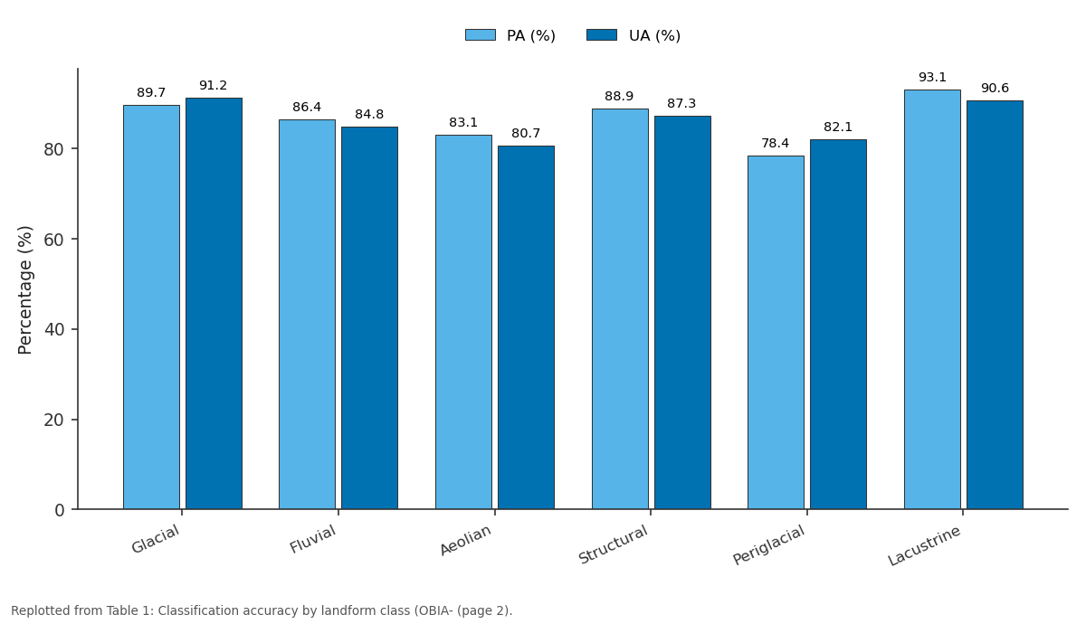
PA (%) and UA (%): Glacial vs Fluvial vs Aeolian vs Structural vs Periglacial
Replotted from Table 1 (page 2) of the original paper. Every bar is the paper's own table value.
View source evidence ↗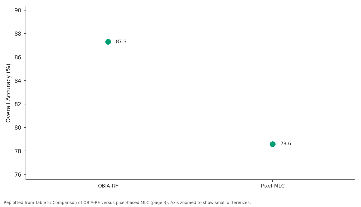
Overall Accuracy (%): OBIA-RF vs Pixel-MLC
Replotted from Table 2 (page 3) of the original paper. Every bar is the paper's own table value.
View source evidence ↗Figures & tables
From the original paper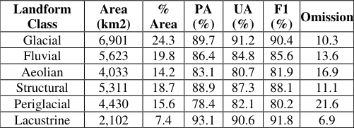 Table 1
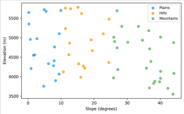 Figure 1
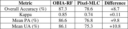 Table 2
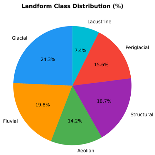 Figure 2
Introduction
The Tibetan Plateau, often called the Third Pole, holds Earth's largest reservoir of ice outside the polar regions and feeds rivers that sustain nearly two billion people downstream [1] . Yet its geomorphology remains incompletely mapped. Traditional landform mapping based on aerial photograph interpretation produces detailed local maps but cannot scale to the plateau's 2.5 million km2 extent [2] . Automated approaches using digital elevation models (DEMs) and satellite imagery offer a solution, but the challenge lies in designing classification schemes and algorithms that capture the diversity of glacial, fluvial, periglacial, aeolian, structural, and lacustrine features present at this scale [3] . Object-based image analysis (OBIA) has gained traction in geomorphological mapping because it classifies meaningful spatial units (objects) rather than individual pixels, thereby incorporating shape, texture, and contextual information that pixel-based methods ignore [4] . OBIA has been successfully applied to landslide mapping in the Himalaya [5] , dune classification in the Sahara [6] , and glacial feature extraction in the European Alps [7] . Applications on the Tibetan Plateau are limited to small test areas, and no OBIA-based landform map covering a regional extent has been published. This research aimed to (i) develop an OBIA workflow for regional landform classification on the Tibetan Plateau, (ii) compare its accuracy against a conventional pixel-based approach, and (iii) identify the terrain derivatives most important for discriminating among the six target landform classes. The work was conducted at the Perth Institute of Climate and Environment, Western Australia [8] .
Spatial Data Processing
The 30 m ASTER GDEM v3 was downloaded from the NASA EarthData portal and mosaicked for the research area. Void-filling used the delta surface fill algorithm.
Twelve terrain derivatives were computed in SAGA-GIS 8.0: slope, aspect, plan curvature, profile curvature, topographic wetness index, terrain ruggedness index, convergence index, valley depth, ridge level, relative slope position, slope length factor, and topographic position index [9] . Sentinel-2 Level-2A surface reflectance data (10 m bands resampled to 30 m) for a cloud-free summer composite (July-August 2022) provided four spectral bands (blue, green, red, NIR) and two derived indices (NDVI, NDWI). All layers were co-registered and stacked into a 18band analysis-ready dataset.
Model Description and Parameterisation
Multi-resolution segmentation in eCognition Developer 10.0 was parameterised through a trial-and-error approach guided by the estimation of scale parameter (ESP) tool [10] . Scale parameters from 20 to 80 were tested in increments of 5, with shape weight 0.3 and compactness 0.5. The optimal SP was determined at 45, producing 14,287 objects with a mean area of 1.99 km2. Object features exported for classification included mean spectral values (4 bands), standard deviation of spectral values, mean terrain derivatives (12 layers), and two geometric features (area and compactness ratio). A random forest (RF) classifier with 500 trees was trained using the randomForest package in R. Training data comprised 420 ground-truth points distributed equally across six classes, identified from high-resolution Google Earth imagery and published geological maps.
Material and Methods Material
The research area covers 28,400 km2 of the central Tibetan Plateau centred on approximately 32.5 N, 87.0 E, spanning elevations from 4,300 m to 6,200 m. Data compilation and analysis were carried out at the Perth Institute of Climate and Environment between February and November 2023. Ground-truth data included 420 training points and 210 independent validation points, allocated using a stratified random sampling strategy. Field photographs from a 2019 expedition by collaborators provided supplementary verification for ambiguous sites.
Methods
Classification accuracy was assessed using an independent validation set of 210 points (35 per class). A confusion matrix yielded overall accuracy (OA), Kappa coefficient, producer accuracy (PA), and user accuracy (UA) per class. Variable importance was ranked using the mean decrease in accuracy metric from the RF model [11] . A pixel-based maximum likelihood classification (MLC) was run on the same input stack for comparison. McNemar's test evaluated whether the OA difference between OBIA-RF and pixel-MLC was statistically significant. All processing used R v4.2.1, SAGA-GIS 8.0, and eCognition Developer 10.0 [12] . Overall accuracy reached 87.3% with a Kappa of 0.85 (Table 1). Lacustrine features were the most accurately classified (PA 93.1%), benefiting from their distinct spectral signature (high NDWI) and flat topographic position. Periglacial landforms had the lowest PA (78.4%), with most misclassifications involving confusion with aeolian deposits where solifluction lobes grade into windblown sand sheets [13] . The scatter plot (Figure 1) reveals clear topographic separation among classes. Plains (low slope, moderate elevation) cluster in the lower left, while mountain features occupy the high-slope domain. Glacial objects span the widest elevation range (4,600-6,200 m), reflecting both valley glaciers and high-altitude cirques [14] .
| Landform Class | Area (km2) | % Area | PA (%) | UA (%) | F1 (%) | Omission |
|---|---|---|---|---|---|---|
| Glacial | 6,901 | 24.3 | 89.7 | 91.2 | 90.4 | 10.3 |
| Fluvial | 5,623 | 19.8 | 86.4 | 84.8 | 85.6 | 13.6 |
| Aeolian | 4,033 | 14.2 | 83.1 | 80.7 | 81.9 | 16.9 |
| Structural | 5,311 | 18.7 | 88.9 | 87.3 | 88.1 | 11.1 |
| Periglacial | 4,430 | 15.6 | 78.4 | 82.1 | 80.2 | 21.6 |
| Lacustrine | 2,102 | 7.4 | 93.1 | 90.6 | 91.8 | 6.9 |
Table text extracted from the original PDF; superscript letters are shown inline. The original table image is below.
View original table image
Results
OBIA-RF outperformed pixel-MLC by 8.7 percentage points in overall accuracy, a difference that was statistically significant (McNemar chi-squared = 14.3, p<0.001). The largest per-class improvements were in aeolian (+13.2%) and periglacial (+11.8%) features, where salt-and-pepper misclassification in the pixel approach was eliminated by object-level smoothing (Table 2) [15] . Glacial landforms made up the largest share (24.3%), followed by fluvial (19.8%) and structural (18.7%). Lacustrine features, though covering just 7.4%, are ecologically significant as they include saline lakes that serve as habitat for migratory birds and as archives of palaeoclimate change (Figure 2) [16] .
| Metric | OBIA-RF | Pixel-MLC | Difference |
|---|---|---|---|
| Overall Accuracy (%) | 87.3 | 78.6 | +8.7 |
| Kappa | 0.85 | 0.74 | +0.11 |
| Mean PA (%) | 86.6 | 76.8 | +9.8 |
| Mean UA (%) | 86.1 | 75.3 | +10.8 |
Table text extracted from the original PDF; superscript letters are shown inline. The original table image is below.
View original table image
Comprehensive Interpretation
Variable importance analysis ranked slope (mean decrease in accuracy = 18.4%), plan curvature (14.7%), and NDVI (11.3%) as the top three discriminators. Spectral bands contributed less individually, but their combined importance (23.1%) exceeded any single terrain derivative. This confirms that integrating spectral and topographic information yields better landform discrimination than either data source alone [17] .
Discussion
The 87.3% overall accuracy is competitive with OBIA landform classifications in other mountain settings. Dragu and colleagues reported 84.1% in the Carpathians [18] , and Eisank and colleagues achieved 86.5% in the Austrian Alps. The Tibetan Plateau presents additional challenges, however: permafrost-related features overlap spectrally with both aeolian and fluvial classes, and the flat interior basins lack the topographic contrast that aids classification in steeper terrain [19] . The scale parameter of 45 produced objects averaging 2 km2, which is appropriate for meso-scale landforms but too coarse to delineate micro-features such as patterned ground or individual moraines. A hierarchical segmentation approach, using a coarser level for regional landform types and a finer level for sub-features, would improve detail without sacrificing classification consistency. This was beyond the scope of the present work but should be a priority for follow-up [20] . A practical limitation is the reliance on the 30 m ASTER GDEM, which introduces vertical errors of 8-12 m on steep slopes. The recently released Copernicus DEM at 30 m, derived from TanDEM-X radar interferometry, offers improved vertical accuracy (approximately 4 m) and could replace ASTER in future iterations. Ground-truth dependence on Google Earth and geological maps rather than field visits also introduces uncertainty, particularly for ambiguous periglacial features [21] .
Conclusion
This research demonstrated that object-based image analysis with a random forest classifier can produce regional-scale landform maps of the Tibetan Plateau at 87.3% accuracy, outperforming pixel-based classification by nearly 9 percentage points. Glacial landforms dominated the research area (24.3%), and lacustrine features were the most accurately classified. Slope, plan curvature, and NDVI were the most informative terrain derivatives. The OBIA workflow provides a reproducible framework for extending landform mapping across the broader plateau, supporting geomorphological inventories, permafrost monitoring, and land-use planning. Future iterations should incorporate higher-resolution DEMs and hierarchical segmentation to capture sub-landform detail.
References
21 in the original paper- Yao T, Thompson L, Yang W. Different glacier status with atmospheric circulations in Tibetan Plateau and surroundings. Nature Climate Change. 2012;2(9):663667.
- Bishop MP, James LA, Shroder JF. Geospatial technologies and digital geomorphological mapping: concepts, issues and research. Geomorphology. 2012;137(1):5-26.
- Hengl T, Reuter HI. Geomorphometry: Concepts, Software, Applications. Elsevier, Amsterdam. 2009;765 pp.
- Blaschke T. Object based image analysis for remote sensing. ISPRS Journal of Photogrammetry and Remote Sensing. 2010;65(1):2-16.
- Martha TR, Kerle N, Jetten V. Characterising spectral, spatial and morphometric properties of landslides for semi-automatic detection using object-oriented methods. Geomorphology. 2010;116(1-2):24-36.
- Hugenholtz CH, Levin N, Barchyn TE. Remote sensing and spatial analysis of aeolian sand dunes: a review and outlook. Earth-Science Reviews. 2012;111(3-4):319334.
- Eisank C, Dragut L, Blaschke T. A generic procedure for semantics-oriented landform classification using object-based image analysis. Geomorphometry. 2011;125-132.
- Florinsky IV. Digital Terrain Analysis in Soil Science and Geology. Elsevier, Amsterdam. 2012;379 pp.
- Wilson JP, Gallant JC. Terrain Analysis: Principles and Applications. John Wiley and Sons, New York. 2000;479 pp.
- Dragut L, Tiede D, Levick SR. ESP: a tool to estimate scale parameter for multiresolution image segmentation of remotely sensed data. International Journal of Geographical Information Science. 2010;24(6):859871.
- Breiman L. Random forests. Machine Learning. 2001;45(1):5-32.
- R Core Team. R: A language and environment for statistical computing. R Foundation, Vienna. 2023.
- French HM. The Periglacial Environment. John Wiley and Sons, Chichester. 2007;458 pp.
- Benn DI, Evans DJA. Glaciers and Glaciation. Hodder Education, London. 2010;802 pp.
- Hay GJ, Castilla G. Geographic object-based image analysis (GEOBIA): a new name for a new discipline. Object-Based Image Analysis. Springer, Berlin. 2008;75-89.
- Zheng M, Xiang J, Wei X. Saline lakes of the QinghaiTibet Plateau: a review. Hydrobiologia. 1993;267(13):23-32.
- Pike RJ, Evans IS, Hengl T. Geomorphometry: a brief guide. Geomorphometry. Elsevier, Amsterdam. 2009;330.
- Dragut L, Blaschke T. Automated classification of landform elements using object-based image analysis. Geomorphology. 2006;81(3-4):330-344.
- Cheng G, Wu T. Responses of permafrost to climate change and their environmental significance. Journal of Geophysical Research. 2007;112(F2):F02S03.
- Burnett C, Blaschke T. A multi-scale segmentation/object relationship modelling methodology for landscape analysis. Ecological Modelling. 2003;168(3):233-249.
- Tadono T, Ishida H, Oda F. Precise global DEM generation by ALOS PRISM. ISPRS Annals. 2014;II4:71-76.