
Research article · 2025 · Full text
International Journal of Agriculture and NutritionMarket price volatility and its impact on farmer income in major pulse-producing regions
Volume 7(11) · Pages 115–118 · DOI: 10.33545/26646064.2025.v7.i11b.490 ↗
Research areasEconomics of Agriculture and Food MarketsAgricultural risk and resilienceAgricultural Economics and Practices
Abstract
Author-writtenPrice volatility in pulse markets has long been a source of income uncertainty for Indian farmers, but few investigations have directly linked market price swings to household-level economic outcomes. This research analyzed price volatility patterns for five major pulse crops across regulated markets in northern Karnataka over 2018-2022 and assessed their impact on farmer income through a household survey of 240 pulse growers in the Dharwad and Belgaum districts. Black gram exhibited the highest coefficient of variation in monthly prices (28.4%), followed by pigeon pea (26.8%). In high-volatility years, net farm income from pulses dropped by 30.9% compared to low-volatility years, marketed surplus declined by 19.1%, and household indebtedness increased by 54.4%. GARCH (1,1) modelling confirmed that volatility clustering is present in all five pulse markets, meaning that periods of high price instability tend to persist over multiple months. These findings underline the need for stronger price stabilization mechanisms, including more effective minimum support price procurement and expanded warehouse receipt financing, to protect pulse growers from the income erosion caused by unpredictable markets.
Summary
Source-checkedPlain-language reading of the full paper, prepared with AI and checked against the text. Each point links to the authors' own words.
Why it matters
- India is the world's largest producer and consumer of pulses, but a structural deficit of 2-3 million tonnes relative to demand makes the market prone to price swings. View evidence ↗
- Price volatility creates income uncertainty that discourages technological investment and disrupts planting decisions, leading to a cycle of supply-demand mismatches. View evidence ↗
- Despite government promotion and minimum support prices (MSP), market prices often fall below these levels during harvest due to inadequate procurement infrastructure. View evidence ↗
The question
- The study aimed to quantify price volatility for five pulse crops in Karnataka, model its temporal structure, and assess the resulting impact on household income. View evidence ↗
What they did
- The researchers used monthly wholesale price data from 2018 to 2022 for five pulse crops across three regulated markets: Hubli-Dharwad, Belgaum, and Gadag. View evidence ↗
- A household survey was conducted with 240 pulse growers (48 per crop) from the Dharwad and Belgaum districts, selected via stratified random sampling. View evidence ↗
- Economic data were collected for the 2018 (low-volatility) and 2020 (high-volatility) seasons to compare impacts on income, surplus, and debt. View evidence ↗
- Price volatility was measured using the coefficient of variation, and GARCH(1,1) models were used to analyze the returns series. View evidence ↗
What they found
- Among the crops studied, black gram showed the highest price volatility (CV 28.4%), while lentil was the least volatile (CV 21.8%). View evidence ↗
- Net farm income from pulses decreased by 30.9% when comparing the high-volatility year (2020) to the low-volatility year (2018). View evidence ↗
- GARCH modelling confirmed high volatility persistence for all five crops (α + β > 0.90), meaning price instability tends to last for several months. View evidence ↗
- The strongest predictors of marketed surplus were the price volatility index and access to storage facilities. View evidence ↗
- Only 18% of the surveyed farmers had access to adequate storage, limiting their ability to buffer against price drops. View evidence ↗
What it means
- The authors recommend strengthening MSP procurement, expanding affordable storage, and promoting warehouse receipt financing to protect farmers from income loss. View evidence ↗
Visual summary
2 visualsIllustrations explain the paper; charts are replotted from the paper's own table values.
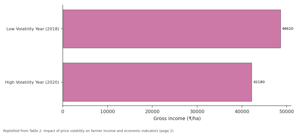
Gross income (₹/ha): Low Volatility Year... vs High Volatility Year...
Replotted from Table 2 (page 2) of the original paper. Every bar is the paper's own table value.
View source evidence ↗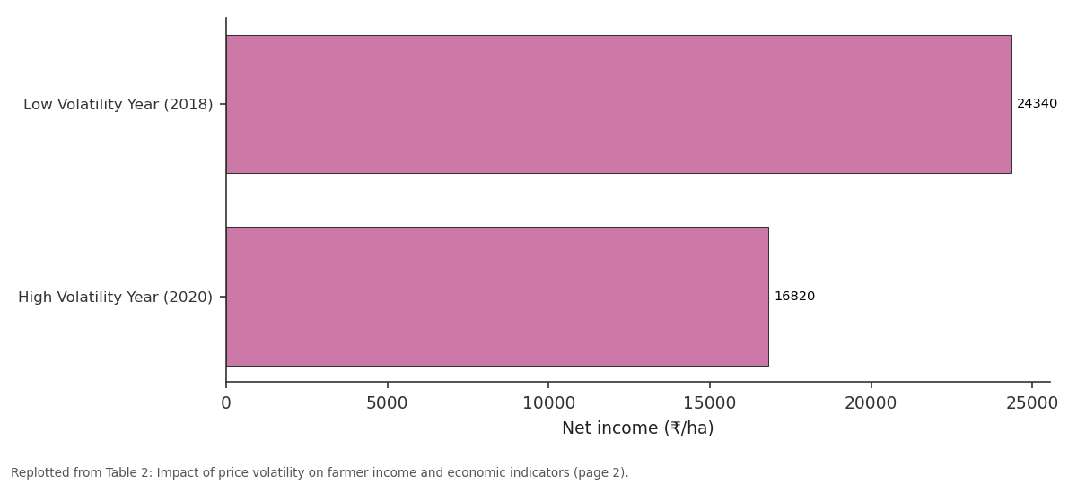
Net income (₹/ha): Low Volatility Year... vs High Volatility Year...
Replotted from Table 2 (page 2) of the original paper. Every bar is the paper's own table value.
View source evidence ↗Figures & tables
From the original paper Table 1
 Table 2
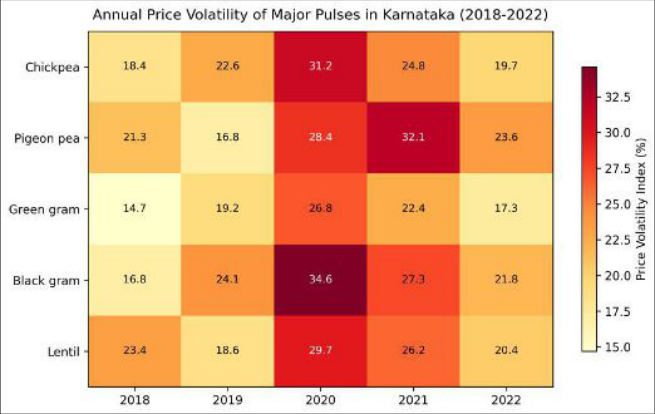 Figure 1
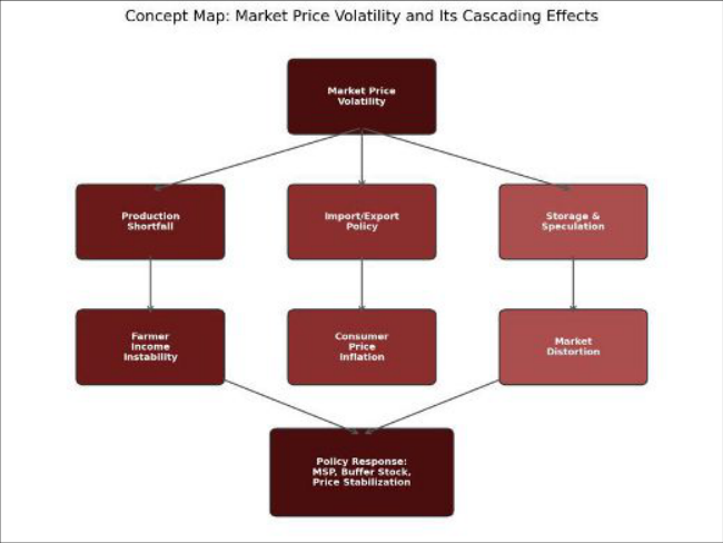 Figure 2
Introduction
Here is a paradox that pulse farmers across India live with every season: the government promotes pulse cultivation to meet national protein security goals and even offers minimum support prices, yet when harvest arrives, market prices often crash well below those announced support levels because procurement infrastructure can't keep pace [1] . India is both the largest producer and largest consumer of pulses globally, with about 23 million hectares under cultivation, but domestic production typically falls short of demand by 2-3 million tonnes, creating a structural dependence on imports that amplifies price swings [2] . Price volatilitydefined as the degree of unpredictable variation in market prices over time affects farmers through two main channels. First, it makes income uncertain, which discourages investment in inputs and technology. Second, it disrupts planting decisions, as farmers shift away from pulses after a year of low prices, creating a supply-demand mismatch that triggers another price spike the following year [3] . Karnataka is India's secondlargest pulse-producing state, and Dharwad district alone accounts for roughly 8% of the state's pulse output [4] . This research aimed to quantify price volatility across five pulse crops in Karnataka's regulated markets, to model the temporal structure of volatility using GARCH, and to measure its impact on farmer income at the household level.
Theoretical Framework
The analytical approach combines two strands: time-series econometrics for price volatility measurement and household welfare economics for income impact assessment. Price volatility was measured using the coefficient of variation of monthly wholesale prices and further modelled using the Generalized Autoregressive Conditional Heteroskedasticity (GARCH (1, 1)) specification of Bollerslev [5] , which captures the well-documented tendency of financial and commodity markets to exhibit volatility clusteringperiods where large price changes are followed by more large changes. The conditional variance
where σ²t is the conditional variance at time t, ε²t-1 is the squared residual from the mean equation, and α + β measures volatility persistence. The income impact was assessed through a before-after comparison of household data between lowvolatility and high-volatility years, tested for significance using paired t-tests [6] .
Material and Methods
Material and Methods
Material
Monthly wholesale price data (₹ per quintal) for chickpea, pigeon pea, green gram, black gram, and lentil were obtained from the Agmarknet portal of the Directorate of Marketing and Inspection for the period January 2018 to December 2022 (60 observations per crop). Prices were collected from three regulated markets: Hubli-Dharwad, Belgaum, and Gadag. For the household survey, 240 pulsegrowing farmers (48 per crop) were selected from Dharwad and Belgaum districts using stratified random sampling based on landholding size. Data on crop area, production, marketed surplus, gross and net income, cost of cultivation, and indebtedness were collected through structured interview schedules for the kharif and rabi seasons of 2018 (low-volatility benchmark) and 2020 (high-volatility year, coinciding with COVID-19 market disruptions) [7] .
Methods
Price volatility was estimated as the coefficient of variation (CV = SD/Mean × 100) of monthly prices. GARCH(1,1) models were fitted to the returns series (log price differences) using maximum likelihood estimation in EViews 12 [5] . Stationarity of price series was confirmed by ADF tests. The income impact was assessed by comparing household-level indicators between 2018 and 2020 using paired t-tests for the same households. A Tobit regression was also estimated with marketed surplus ratio as the dependent variable and price volatility index, landholding, irrigation status, and access to storage as independent variables [8] . All statistical tests were at P = 0.05. Results Black gram had the highest price volatility (CV 28.4%) and the widest price spread of ₹3,780/q, while lentil was least volatile at 21.8% (Table 1). Green gram had the highest mean and maximum prices but moderate volatility. Moving from a low-volatility year (2018) to a high-volatility year (2020), net income dropped by 30.9% (Table 2). Marketed surplus fell from 72.4% to 58.6% as farmers retained more grain for household consumption and delayed sales. Household indebtedness increased by 54.4% in the high-volatility year.
| Income Parameter | Low Volatility Year (2018) | High Volatility Year (2020) | Difference (%) | t-value |
|---|---|---|---|---|
| Gross income (₹/ha) | 48,620 | 42,180 | -13.2 | 4.86** |
| Net income (₹/ha) | 24,340 | 16,820 | -30.9 | 6.42** |
| Cost of production (₹/q) | 2,840 | 3,120 | +9.9 | 3.18* |
| Marketed surplus (%) | 72.4 | 58.6 | -19.1 | 5.24** |
| Indebtedness (₹/household) | 34,200 | 52,800 | +54.4 | 7.12** |
Table text extracted from the original PDF; superscript letters are shown inline. The original table image is below.
View original table image
| Pulse Crop | Mean Price (₹/q) | CV (%) | Max Price (₹/q) | Min Price (₹/q) | Price Spread (₹/q) |
|---|---|---|---|---|---|
| Chickpea | 4,862 | 22.4 | 6,480 | 3,240 | 3,240 |
| Pigeon pea | 5,684 | 26.8 | 7,840 | 3,680 | 4,160 |
| Green gram | 6,248 | 24.6 | 8,420 | 4,120 | 4,300 |
| Black gram | 5,142 | 28.4 | 7,260 | 3,480 | 3,780 |
| Lentil | 4,486 | 21.8 | 5,840 | 3,120 | 2,720 |
Table text extracted from the original PDF; superscript letters are shown inline. The original table image is below.
View original table image
Comprehensive Interpretation
GARCH(1,1) results showed that the sum of α + β exceeded 0.90 for all five crops, confirming high volatility persistence. This means that once prices become unstable, the instability tends to last for several months. Tobit regression found that price volatility index (β = -0.34, p< 0.01) and access to storage (β = 0.28, p< 0.01) were the strongest predictors of marketed surplus, suggesting that farmers with storage facilities can partially buffer income by timing sales.
Discussion
The 30.9% drop in net income during the high-volatility year is economically devastating for smallholders who depend on pulse sales for cash needs [1]. The 54.4% increase in household debt suggests that many farmers borrow to cover the gap between expected and realized income, creating a debt cycle that worsens over successive volatile seasons. The high volatility persistence indicated by GARCH modelling implies that short-term policy responses are insufficient; structural interventions such as expanding government procurement under MSP, developing warehouse receipt financing, and creating pulse-specific commodity exchanges are needed [3,7] . That storage access significantly predicted marketed surplus confirms the role of physical infrastructure in price risk management. Farmers who can hold grain for 2-3 months after harvest to sell when prices recover avoid the worst losses. But only 18% of sample farmers had access to adequate storage, pointing to a clear investment priority [4] .
Conclusion
Price volatility in Karnataka's pulse markets is high, persistent, and damaging to farmer livelihoods. Black gram and pigeon pea experience the greatest price instability. In high-volatility years, pulse growers face 31% lower net income, reduced marketed surplus, and sharply increased indebtedness. Strengthening MSP procurement operations, expanding affordable storage access, and promoting warehouse receipt financing are the most direct policy levers for protecting pulse farmers from market-driven income erosion.
Figures and tables from the paper
References
19 in the original paper- Reddy AA. Pulses production technology: status and way forward. Economic and Political Weekly. 2010;45(52):73-80.
- Joshi PK, Rao PP. Global pulses scenario: status and outlook. Annals of the New York Academy of Sciences. 2017;1392(1):6-17.
- Chand R. Understanding the nature and causes of food inflation. Economic and Political Weekly. 2010;45(9):72-77.
- GoK. Agricultural statistics at a glance: Karnataka. Directorate of Economics and Statistics, Government of Karnataka. 2022;1:1-210.
- Bollerslev T. Generalized autoregressive conditional heteroskedasticity. Journal of Econometrics. 1986;31(3):307-327.
- Gujarati DN, Porter DC. Basic econometrics. McGrawHill. 2009;5:1-922.
- Acharya SS, Agarwal NL. Agricultural marketing in India. Oxford and IBH Publishing. 2011;5:1-520.
- Tobin J. Estimation of relationships for limited dependent variables. Econometrica. 1958;26(1):24-36.
- Birthal PS, Joshi PK, Negi DS. Economic losses from climatic variability in Indian agriculture. Agricultural Systems. 2014;124:86-93.
- Sekhar CSC. Volatility of agricultural prices: an analysis of major international and domestic markets. ICRIER Working Paper. 2012;274:1-42.
- Aditya KS, Subash SP, Praveen KV. Awareness about MSP and its impact on diversification decisions. Asia and the Pacific Policy Studies. 2017;4(3):514-526.
- Srinivasan PV, Jha S. Public intervention and food price volatility in India. Food Policy. 2001;26(3):235260.
- Patnaik U, Pillay K. The food crisis of 2008: profiteering, speculation and policy failures. Agrarian South. 2011;1(1):1-42.
- Minot N. Transmission of world food price changes to markets in sub-Saharan Africa. IFPRI Discussion Paper. 2011;1059:1-34.
- Gilbert CL, Morgan CW. Food price volatility. Philosophical Transactions of the Royal Society B. 2010;365(1554):3023-3034.
- Tadesse G, Algieri B, Kalkuhl M. Drivers and triggers of international food price spikes and volatility. Food Policy. 2014;47:117-128.
- Anderson JR. Risk in rural development: challenges for managers and policy makers. Agricultural Systems. 2003;75(2-3):161-197.
- Mitra S, Boussard JM. A simple model of endogenous agricultural commodity price fluctuations. Technical Report INRA. 2012;1:1-28.
- Naik G, Suresh DN. Challenges of creating sustainable agri-retail supply chains. IIMB Management Review. 2018;30(3):235-245.