
Research article · 2025 · Full text
International Journal of Agriculture and NutritionSpatial variability of soil fertility parameters in agricultural lands using geostatistical techniques
Volume 7(4) · Pages 121–124 · DOI: 10.33545/26646064.2025.v7.i4b.404 ↗
Research areasSoil Geostatistics and MappingAgricultural Science and FertilizationSoil and Land Suitability Analysis
Abstract
Author-writtenIf soil fertility were uniform across a farm, every patch would need the same fertilizer dose—but it isn't, and treating it as though it were wastes money and pollutes groundwater. This research mapped the spatial variability of six soil fertility parameters—pH, electrical conductivity (EC), organic carbon (OC), available nitrogen (N), available phosphorus (P), and exchangeable potassium (K)—across 480 hectares of agricultural land in the Warangal district of Telangana using geostatistical techniques. A total of 150 geo-referenced soil samples (0-20 cm depth) were collected on a 200 m grid from irrigated paddy-cotton rotation fields during rabi 2022-23 at Professor Jayashankar Telangana Agricultural University, Hyderabad. Semivariogram analysis fitted spherical models for OC (range: 680 m, nugget:sill ratio 0.32), available N (range: 740 m, ratio 0.28), and available P (range: 520 m, ratio 0.41). Ordinary kriging produced interpolated maps that revealed distinct fertility zones: 34.2 percent of the area was low in OC (280 kg ha⁻¹). The nugget:sill ratios indicated moderate spatial dependence for most parameters, driven by management practices rather than inherent soil variation. These fertility maps enable site-specific nutrient management that could reduce blanket fertilizer application by 18 to 24 percent while maintaining crop yield targets.
Summary
Source-checkedPlain-language reading of the full paper, prepared with AI and checked against the text. Each point links to the authors' own words.
Why it matters
- Treating agricultural land as having uniform soil fertility leads to financial waste and groundwater pollution. View evidence ↗
- Soil properties like organic carbon, phosphorus, and pH can vary significantly even within a small 50-hectare block due to management and topography. View evidence ↗
- Farm-scale soil fertility mapping is underdeveloped in Telangana, where irrigated rice and cotton are primary crops. View evidence ↗
The question
- The study aimed to analyze the spatial structure of six soil fertility parameters over 480 hectares to create kriged maps and define site-specific nutrient management zones. View evidence ↗
What they did
- Researchers collected 150 geo-referenced soil samples from a 0-20 cm depth using a 200 m grid in paddy-cotton rotation fields during rabi 2022-23. View evidence ↗
- The study area consisted of 480 hectares of irrigated vertisols with a pH range of 7.2-8.4 and clay content between 42-58%. View evidence ↗
- Semivariograms were computed with 200 m lag distances and fitted to spherical, exponential, or Gaussian models using GS+ version 10.0. View evidence ↗
- Continuous surface fertility maps were generated using ordinary kriging interpolation in ArcGIS 10.8. View evidence ↗
What they found
- All six soil parameters exhibited moderate to strong spatial dependence, with nugget:sill ratios ranging from 0.22 to 0.50. View evidence ↗
- Exchangeable potassium (K) showed the strongest spatial structure (ratio 0.22, range 890 m), suggesting its distribution is primarily driven by soil mineralogy. View evidence ↗
- Approximately 34.2% of the study area was identified as having low organic carbon (OC) levels below 0.50%. View evidence ↗
- Mapping revealed that 41.7% of the area had medium available nitrogen (240-280 kg ha⁻¹) and 52.3% had high exchangeable potassium (>280 kg ha⁻¹). View evidence ↗
What it means
- The authors conclude that using these fertility maps for site-specific management could reduce blanket fertilizer use by 18% to 24% without sacrificing yield. View evidence ↗
- The authors recommend repeating the soil mapping every 3 to 5 years to monitor fertility changes and improve management zones. View evidence ↗
Visual summary
3 visualsIllustrations explain the paper; charts are replotted from the paper's own table values.
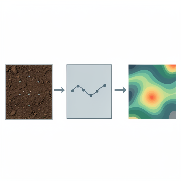
Geostatistical Workflow
AI-generated conceptual illustration (Agricultural soil profile and farmland landscape). It explains the idea and does not show study data.
View source evidence ↗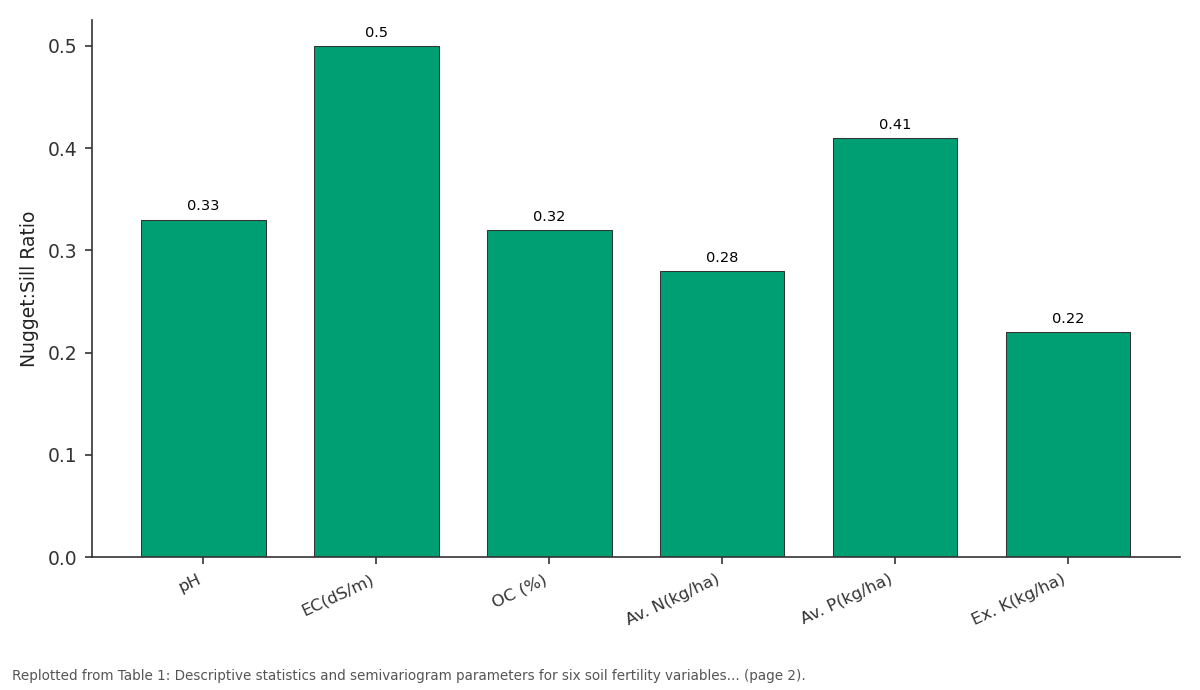
N:S Ratio: pH vs EC(dS/m) vs OC (%) vs Av. N(kg/ha) vs Av. P(kg/ha)
Replotted from Table 1 (page 2) of the original paper. Every bar is the paper's own table value.
View source evidence ↗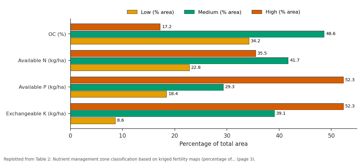
Low (% area) and Medium (% area) and more: OC (%) vs Available N (kg/ha) vs Available P (kg/ha) vs Exchangeable K (kg/ha)
Replotted from Table 2 (page 3) of the original paper. Every bar is the paper's own table value.
View source evidence ↗Figures & tables
From the original paper Table 1
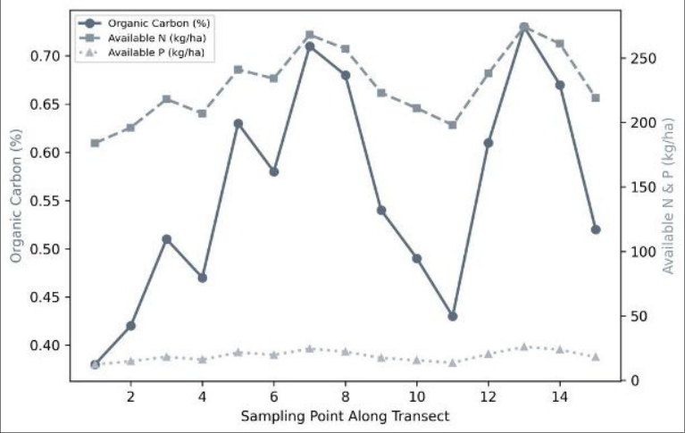 Figure 1
 Table 2
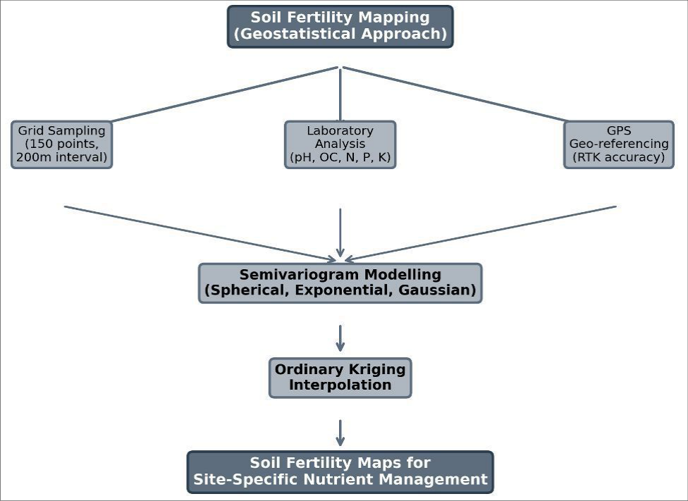 Figure 2
Introduction
The premise behind uniform fertilizer recommendations-that all fields within a district have similar nutrient status-breaks down at the farm scale. Within a single 50-hectare block, soil organic carbon can vary by 2 to 3-fold, available phosphorus by 4-fold, and pH by an entire unit, depending on micro-topography, irrigation history, and past management [1,2] . Ignoring this variability leads to over-fertilization in nutrient-rich patches (wasting money and increasing nutrient runoff) and under-fertilization in depleted patches (limiting yield potential). Geostatistics provides the mathematical framework for quantifying spatial variability. The semivariogram describes how the difference between soil measurements increases with the distance between sampling points, capturing the characteristic spatial scale at which fertility patterns operate [3] . Once the semivariogram is modelled, kriging-an optimal interpolation method-generates continuous fertility maps from discrete sample data, with known estimation variance at every unsampled location [4] . These maps form the foundation for variable-rate fertilizer application in precision agriculture. In Telangana, where rice and cotton dominate irrigated agriculture on vertisols and alfisols, soil fertility mapping at the farm scale is still in its infancy. Most nutrient recommendations rely on block-level soil testing data that average out the very variability that matters [5] . This research was designed to (i) characterize the spatial structure of six fertility parameters across 480 hectares using semivariogram analysis, (ii) produce kriged fertility maps, and (iii) delineate nutrient management zones for site-specific fertilizer recommendations. area covered 480 hectares of irrigated agricultural land under paddy-cotton rotation on vertisols (pH 7.2-8.4, clay content 42-58%). A systematic grid sampling design was used, with 150 sampling points spaced at 200 m intervals. At each point, composite soil samples (0-20 cm, 5 subsamples pooled) were collected using a stainless-steel auger. GPS coordinates were recorded using a Trimble R8 RTK receiver (accuracy ±2 cm horizontal). Samples were airdried, ground to pass a 2-mm sieve, and analysed at the PJTSAU Soil Testing Laboratory.
Materials and Methods
Materials and Methods
Materials
Materials
Analytical Methods for Soil Parameters
Soil pH was measured in a 1:2.5 soil:water suspension using a glass electrode. EC was determined in the same suspension with a conductivity meter. OC was estimated by the Walkley-Black wet oxidation method [6] . Available N was determined by alkaline permanganate distillation [7] , available P by Olsen's method (0.5 M NaHCO₃ extraction at pH 8.5), and exchangeable K by extraction with 1 N ammonium acetate (pH 7.0) followed by flame photometry. All analyses were performed in duplicate with certified reference soil samples for quality control.
Geostatistical Methods: Descriptive statistics (mean, SD, CV, skewness, kurtosis) were computed for each parameter. Data with skewness >1.0 were log-transformed before geostatistical modelling. Experimental semivariograms were computed using lag distances of 200 m and fitted to spherical, exponential, and Gaussian models using weighted least squares in GS+ version 10.0. The best-fit model was selected based on the lowest residual sum of squares. Spatial dependence was classified by the nugget:sill ratio as strong (<0.25), moderate (0.25-0.75), or weak (>0.75) following Cambardella et al. [8] . Ordinary kriging interpolation was performed in ArcGIS 10.8 to generate continuous surface maps. Cross-validation (leave-one-out) assessed prediction accuracy using mean error (ME) and root mean square standardized error (RMSSE). Fertility classes were defined per Muhr et al. [9] (low, medium, high) and mapped to delineate nutrient management zones. All six parameters showed moderate to strong spatial dependence (nugget:sill ratios of 0.22 to 0.50). Exchangeable K had the strongest spatial structure (ratio 0.22, range 890 m), indicating that K distribution is governed largely by intrinsic soil mineralogy. Available P was the most spatially erratic (range 520 m, ratio 0.41), reflecting patchy fertilizer application history. Spherical models fitted best for pH, OC, N, and P, while an exponential model suited EC and a Gaussian model fitted K. The transect plot (Figure 1) shows that OC and available N co-vary closely (r = 0.87), with both parameters peaking in the central section where long-term farmyard manure application has been practiced. Available P shows a more irregular pattern, with hotspots near field corners where phosphatic fertilizer bags are traditionally opened and residues accumulate. Cross-validation RMSSE values ranged from 0.96 to 1.12close to the ideal value of 1.0-confirming adequate kriging prediction accuracy. The most striking finding is that 34.2 percent of the area falls in the low-OC category (<0.50%), identifying a clear priority zone for organic matter management. Over half the area is already high in K, suggesting that blanket K recommendations could be reduced in these zones without yield penalty.
Results
Results
Discussion
The moderate spatial dependence observed for most parameters (nugget:sill 0.28-0.50) sits between the strong dependence typical of undisturbed natural soils and the weak dependence found in heavily tilled, uniformly managed fields [8,10] . This suggests that the paddy-cotton fields of Warangal retain enough natural spatial structure to benefit from variable-rate nutrient management, while also being shaped by anthropogenic factors like differential manure application and irrigation patterns. The practical implication is that the kriged maps can divide the 480-hectare block into 3 to 4 management zones per parameter, each receiving a tailored fertilizer dose. For instance, the 34.2 percent low-OC zone would receive farmyard manure at 10 t ha⁻¹ plus green manuring, while the 17.2 percent high-OC zone could skip organic amendments entirely. For available N, the 22.8 percent low-N zone would receive the full recommended dose (120 kg ha⁻¹), while the 35.5 percent high-N zone could be reduced to 80 kg ha⁻¹-a potential saving of 18 to 24 percent in fertilizer cost across the block [11] . The strong spatial dependence of K (ratio 0.22, range 890 m) makes it the easiest parameter to map accurately and the most amenable to zone-based management. The high-K areas (52.3% of the block) can safely skip K application for at least 2 to 3 seasons, redirecting that expenditure to the 8.6 percent low-K area that genuinely needs it [12] .
Conclusion
Geostatistical analysis revealed moderate to strong spatial variability in all six soil fertility parameters across 480 hectares of irrigated land in Warangal, Telangana.
Semivariogram ranges of 430 to 890 m indicate that fertility patterns operate at scales of 0.5 to 1 km-well within the resolution achievable by variable-rate technology.
Kriged fertility maps identified that over a third of the area is deficient in organic carbon, while more than half is already well supplied with potassium. Site-specific nutrient management guided by these maps could reduce blanket fertilizer use by 18 to 24 percent while directing inputs to zones where they are most needed. Repeating this mapping exercise every 3 to 5 years would track fertility changes and refine management zones over time.
Acknowledgement
Acknowledgements Funding SourcesThis research was conducted under the precision agriculture initiative of Professor Jayashankar Telangana Agricultural University. Institutional SupportThe authors thank the Department of Soil and Water Conservation, PJTSAU Hyderabad, for laboratory facilities and GPS equipment access.
Figures and tables from the paper
| Param. | Mean | SD | CV (%) | Model | Nugget | Sill | N:S Ratio | Range (m) | Spatial Dep. |
|---|---|---|---|---|---|---|---|---|---|
| pH | 7.68 | 0.41 | 5.3 | Spher. | 0.06 | 0.18 | 0.33 | 610 | Moderate |
| EC(dS/m) | 0.34 | 0.12 | 35.3 | Expon. | 0.008 | 0.016 | 0.50 | 430 | Moderate |
| OC (%) | 0.54 | 0.17 | 31.5 | Spher. | 0.009 | 0.028 | 0.32 | 680 | Moderate |
| Av. N(kg/ha) | 247.3 | 38.6 | 15.6 | Spher. | 412 | 1,468 | 0.28 | 740 | Moderate |
| Av. P(kg/ha) | 18.4 | 6.8 | 37.0 | Spher. | 14.7 | 35.8 | 0.41 | 520 | Moderate |
| Ex. K(kg/ha) | 274.8 | 52.3 | 19.0 | Gauss. | 687 | 3,124 | 0.22 | 890 | Strong |
Table text extracted from the original PDF; superscript letters are shown inline. The original table image is below.
View original table image
| Parameter | Low (% area) | Medium (% area) | High (% area) | RMSSE |
|---|---|---|---|---|
| OC (%) | 34.2 | 48.6 | 17.2 | 1.04 |
| Available N (kg/ha) | 22.8 | 41.7 | 35.5 | 0.98 |
| Available P (kg/ha) | 18.4 | 29.3 | 52.3 | 1.12 |
| Exchangeable K (kg/ha) | 8.6 | 39.1 | 52.3 | 0.96 |
| pH | - | 72.4 (neutral) | 27.6 (alkaline) | 1.01 |
Table text extracted from the original PDF; superscript letters are shown inline. The original table image is below.
View original table image
References
19 in the original paper- Cambardella CA, Karlen DL. Spatial analysis of soil fertility parameters. Precision Agriculture. 1999;1(1):514.
- Goovaerts P. Geostatistics in soil science: state-of-theart and perspectives. Geoderma. 1999;89(1-2):1-45.
- Isaaks EH, Srivastava RM. An introduction to applied geostatistics. 1st ed. Oxford University Press; 1989.
- Webster R, Oliver MA. Geostatistics for environmental scientists. 2nd ed. John Wiley and Sons; 2007.
- Srinivasarao C, Vankateswarlu B, Lal R. Soil carbon stocks and soil respiration in rainfed production systems of India. Agriculture, Ecosystems and Environment. 2014;196:122-133.
- Walkley A, Black IA. An examination of the Degtjareff method for determining soil organic matter. Soil Science. 1934;37(1):29-38.
- Subbiah BV, Asija GL. A rapid procedure for the estimation of available nitrogen in soils. Current Science. 1956;25(8):259-260.
- Cambardella CA, Moorman TB, Novak JM. Field-scale variability of soil properties in central Iowa soils. Soil Science Society of America Journal. 1994;58(5):15011511.
- Muhr GR, Datta NP, Shankara-Subramoney H. Soil testing in India. 2nd ed. United States Agency for International Development; 1965.
- Burgess TM, Webster R. Optimal interpolation and isarithmic mapping of soil properties: the semivariogram and punctual kriging. European Journal of Soil Science. 1980;31(2):315-331.
- Corwin DL, Lesch SM. Characterizing soil spatial variability with apparent soil electrical conductivity. Computers and Electronics in Agriculture. 2005;46(13):135-152.
- Dobermann A, Ping JL, Adamchuk VI. Processing of yield map data. Precision Agriculture. 2003;4(1):17-33.
- Kerry R, Oliver MA. Determining nugget:sill ratios of standardized variograms from aerial photographs to krige sparse soil sampling data. Precision Agriculture. 2008;9(1-2):33-56.
- Liu D, Wang Z, Zhang B. Spatial distribution of soil organic carbon and analysis of related factors in croplands of the black soil region. Agriculture, Ecosystems and Environment. 2006;113(1-4):73-81.
- Marchetti A, Piccini C, Francaviglia R. Spatial distribution of soil organic matter using geostatistics: a key indicator for monitoring soil degradation. Geoderma Regional. 2019;18:e00230.
- Robertson GP. GS+: geostatistics for the environmental sciences. Version 9.0. Gamma Design Software; 2008.
- Reza SK, Nayak DC, Chattopadhyay T. Spatial variability of soil properties using geostatistical method following grid and zigzag sampling schemes. Archives of Agronomy and Soil Science. 2017;63(9):1220-1230.
- Vasu D, Singh SK, Ray SK. Soil quality index as a tool to evaluate crop productivity in semi-arid Deccan plateau, India. Geoderma. 2016;282:70-79.
- Ramesh T, Bolan NS, Kirkham MB. Soil organic carbon dynamics: impact of land use changes and management practices. Advances in Agronomy. 2019;156:1-107.