
Research article · 2026 · Full text
International Journal of Geography Geology and EnvironmentRemote Sensing Based Monitoring and Estimation of Lacustrine Chlorophyll-a Concentration in South Tamil Nadu: A Case Study
Volume 8(4) · Pages 28–37 · DOI: 10.22271/27067483.2026.v8.i4a.507 ↗
Research areasWater Quality Monitoring TechnologiesAquatic Ecosystems and Phytoplankton DynamicsWater Quality and Pollution Assessment
Abstract
Author-writtenLacustrine water bodies are vital for domestic, agricultural, and economic activities, necessitating continuous water quality monitoring for their sustainable management, and the study focuses on inland water bodies from eleven southern districts of Tamil Nadu. Among various water quality parameters, chlorophyll-a (Chl-a) serves as a key indicator of algal biomass and ecosystem productivity, playing a crucial role in assessing eutrophication and water health. Traditional in-situ monitoring methods for Chl-a are often labour-intensive, time-consuming, and expensive. Remote sensing offers an efficient alternative, enabling large-scale and frequent assessments of Chl-a dynamics. This study employs Sentinel-2 satellite imagery to estimate and monitor Chl-a concentration in selected lacustrine environments of South Tamil Nadu. The study aims to improve understanding of spatial and temporal variations in Chl-a levels through the use of remote sensing techniques, allowing for data-driven decision-making for sustainable water resource management. Remote sensing technology is excellent for monitoring water quality.
Summary
Source-checkedPlain-language reading of the full paper, prepared with AI and checked against the text. Each point links to the authors' own words.
Why it matters
- Lacustrine water bodies are essential for economic, agricultural, and domestic use, making continuous water quality monitoring necessary for sustainable management. View evidence ↗
- Chlorophyll-a (Chl-a) is a critical indicator used to assess water health and eutrophication because it reflects ecosystem productivity and algal biomass. View evidence ↗
- Traditional methods for monitoring Chl-a are often too expensive, time-consuming, and labor-intensive for frequent use. View evidence ↗
The question
- The study aims to use Sentinel-2 satellite imagery to monitor Chl-a concentrations across eleven districts in South Tamil Nadu to address the lack of continuous monitoring in inland water bodies. View evidence ↗
What they did
- The researchers identified 33 inland water bodies, each with a surface area exceeding 3 square kilometers, for the study. View evidence ↗
- Seasonal analysis was conducted using Sentinel-2B MSI data from December 2024 (winter) and March 2025 (summer). View evidence ↗
- To analyze land use and land cover (LULC), a 1-kilometer buffer was applied around each lake using Google Earth Engine. View evidence ↗
What they found
- Across all selected periods (Winter 2024 and Summer 2025), the calculated Chl-a concentrations ranged from 4.5 mg/m³ to 193.34 mg/m³. View evidence ↗
- The most significant seasonal declines in Chl-a (over 65%) were observed in the Palar Dam, Palakudi, and Ovalur tanks. View evidence ↗
- Larger reservoirs, including Hope Lake, Kodayar, and Vaigai, showed more modest Chl-a reductions of approximately 30-40%. View evidence ↗
- Statistical analysis revealed that rainfall alone does not linearly influence Chl-a variability, showing a very weak and insignificant correlation (r = -0.06, p = 0.808). View evidence ↗
- Land use significantly influenced Chl-a dynamics, with grasslands (r = +0.554) and wetlands (r = +0.583) positively correlating with Chl-a increases, while tree-covered catchments showed a moderate negative correlation (r = -0.489). View evidence ↗
What it means
- The authors conclude that land use patterns within lake catchments are a significant influence on the seasonal dynamics of Chl-a. View evidence ↗
- The authors recommend incorporating land use and land cover (LULC) data into remote sensing assessments to improve water quality monitoring. View evidence ↗
Visual summary
2 visualsIllustrations explain the paper; charts are replotted from the paper's own table values.
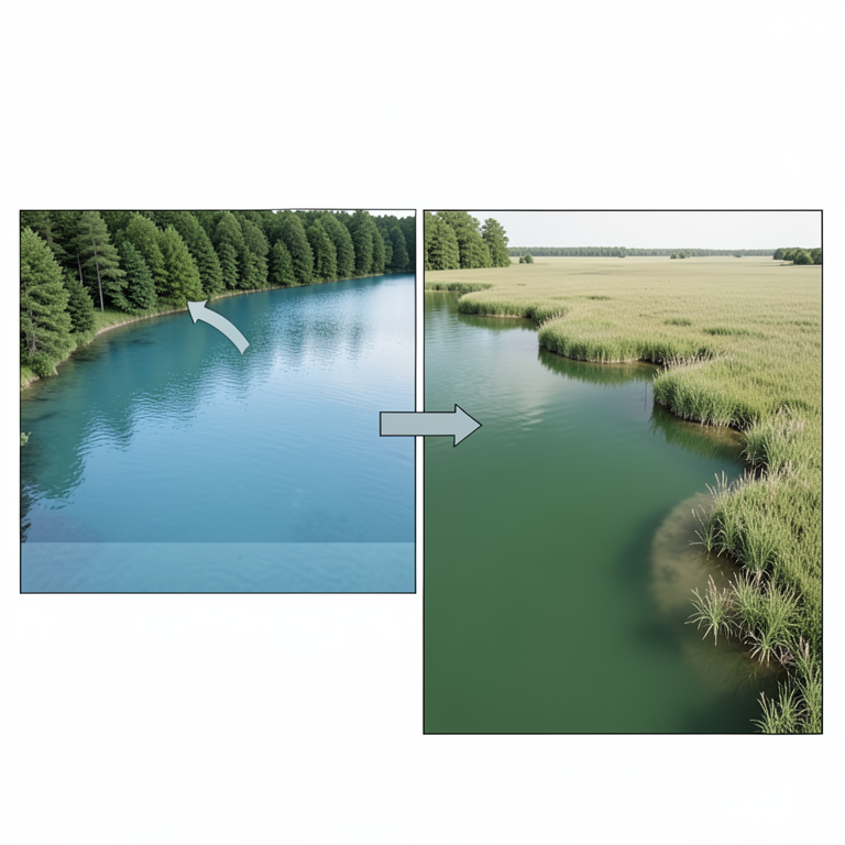
LULC Influence on Chl-a
AI-generated conceptual illustration (A freshwater lake in South Tamil Nadu surrounded by diverse land cover). It explains the idea and does not show study data.
View source evidence ↗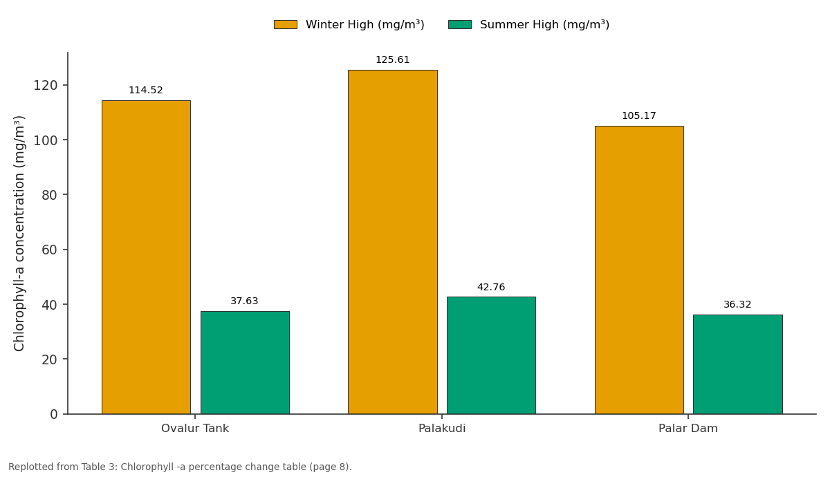
Winter High (mg/m³) and Summer High (mg/m³): Ovalur Tank vs Palakudi vs Palar Dam
Replotted from Table 3 (page 8) of the original paper. Every bar is the paper's own table value.
View source evidence ↗Figures & tables
From the original paper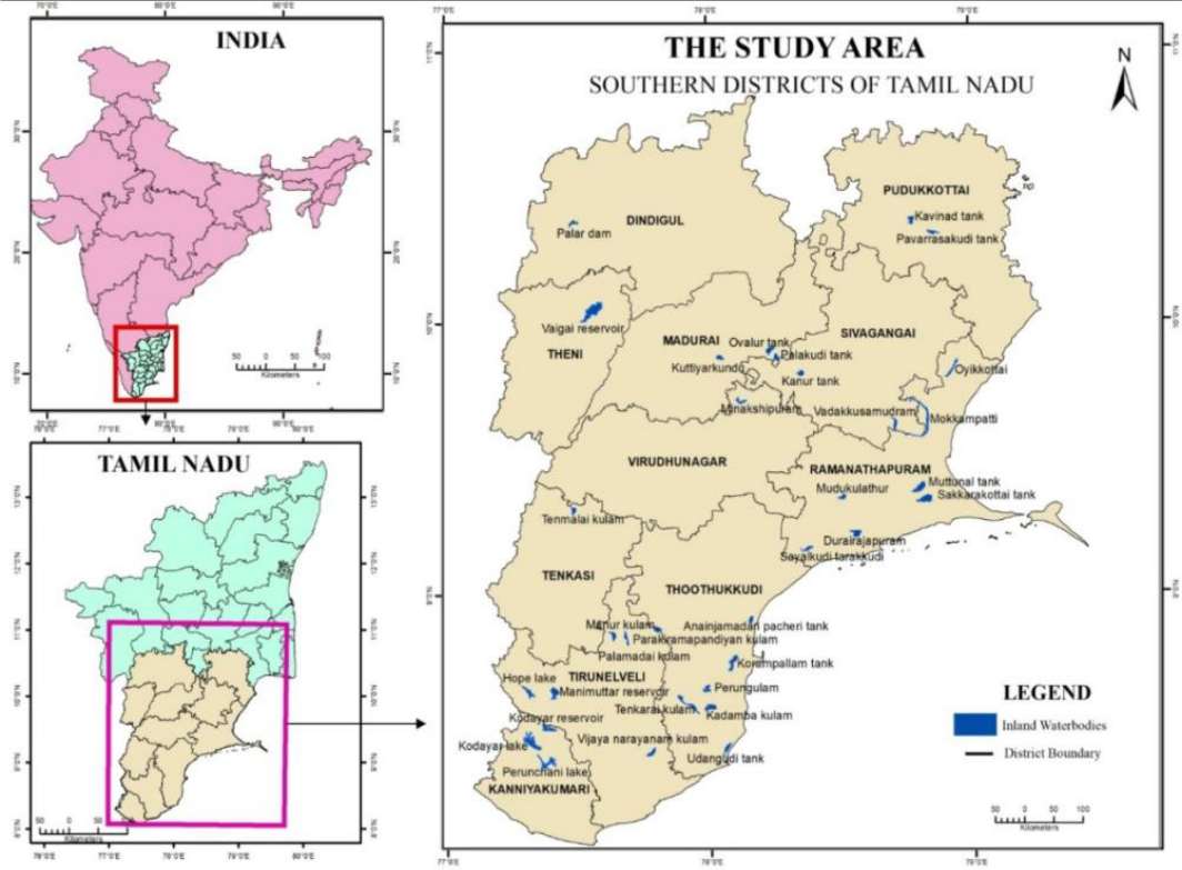 Figure 1
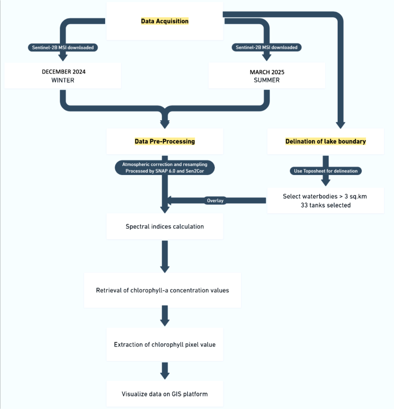 Figure 2
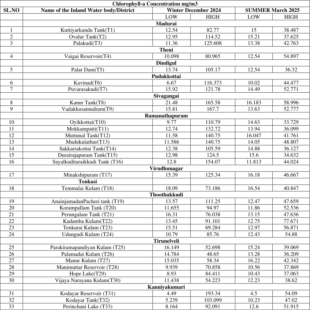 Table 2
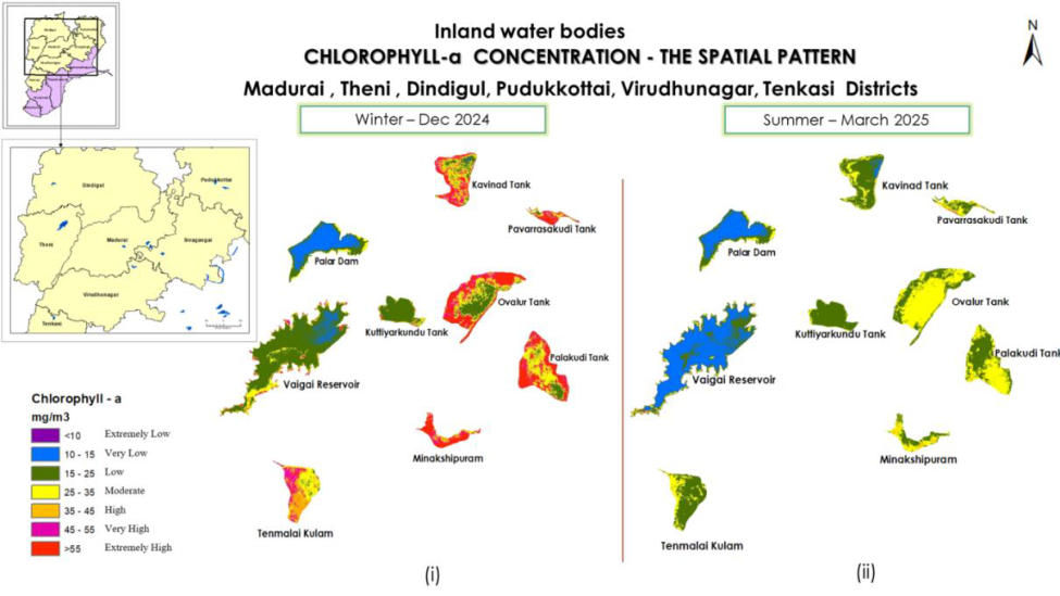 Figure 3
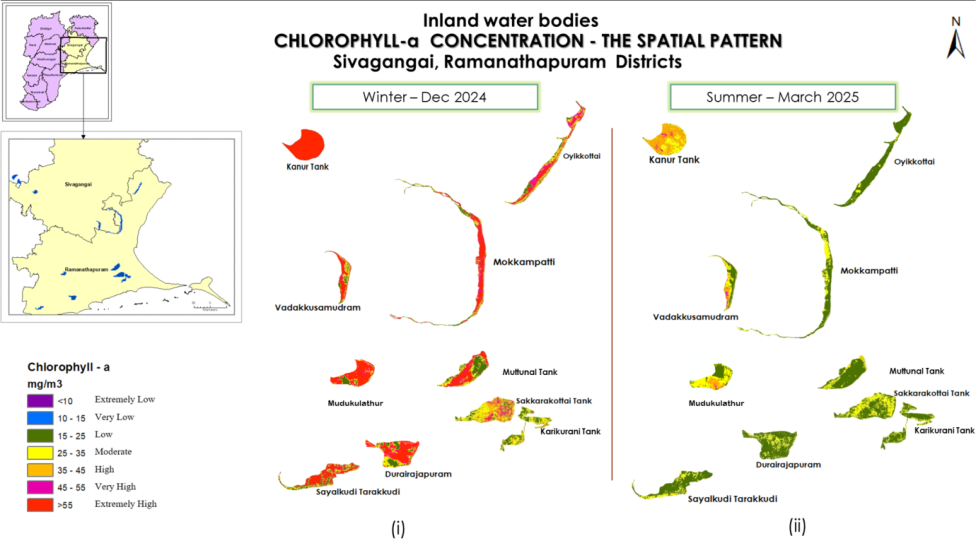 Figure 3
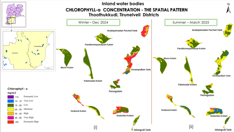 Figure 3
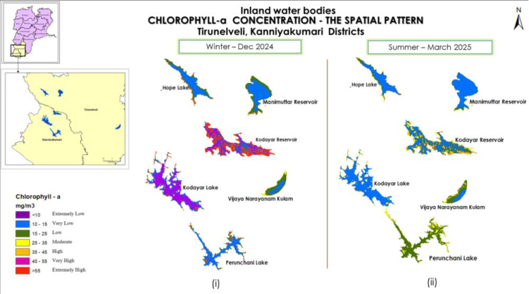 Figure 3
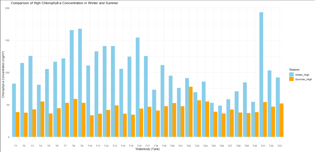 Figure 4
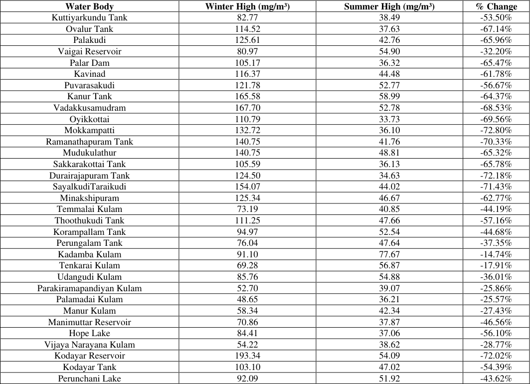 Table 3
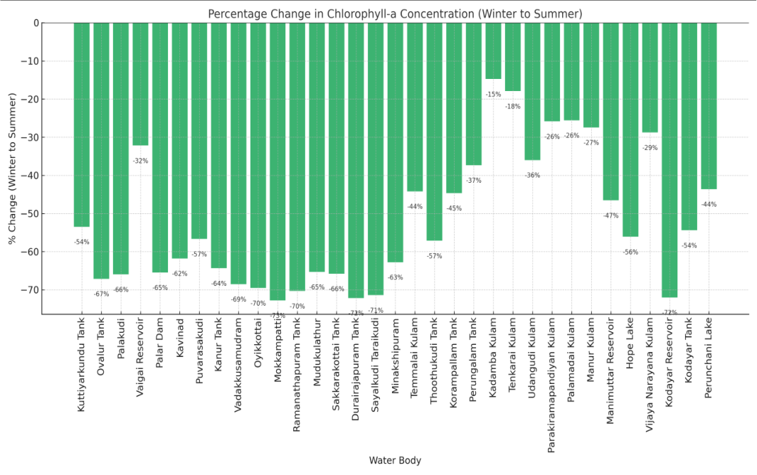 Figure 5
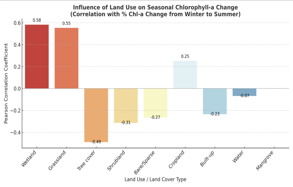 Figure 6
Introduction
Water bodies are highly vulnerable to ecological changes due to natural processes and human interventions, necessitating continuous monitoring of their water quality. Excessive algal growth, often indicated by elevated Chl-a concentrations, can lead to severe water quality issues such as oxygen depletion, odor, and the formation of harmful algal blooms (HABs), which pose significant threats to aquatic ecosystems and public health [1] . Traditional methods for measuring Chl-a concentration rely on in-situ sampling and laboratory analysis, which are often labor-intensive, time-consuming, and expensive [2] . These challenges have led to the increased adoption of remote sensing techniques as a viable alternative for large-scale and cost-effective water quality assessment. The availability of high-resolution Sentinel-2 satellite imagery provides an opportunity to monitor Chl-a concentration efficiently, offering extensive spatial and temporal coverage. Remote sensing facilitates the estimation of water quality parameters using spectral reflectance, allowing researchers to track changes in Chl-a dynamics over time [3] . Several studies worldwide have demonstrated the potential of remote sensing techniques for monitoring Chl-a concentration and understanding algal bloom dynamics. Research on Lake Winnipeg, North America, analyzed spatial and temporal variability in algal blooms using satellite-derived Chl-a indices, integrating ESA's MERIS mission data from 2002 to 2011 [4] . Similarly, studies in Jordan evaluated remote sensing data accuracy for Chl-a estimation, developing predictive models validated with Sentinel-2 surface reflectance data [5] . Additional research from China, Europe, and Africa has further highlighted the effectiveness of remote sensing for Chl-a monitoring, emphasizing the importance of integrating satellite-based techniques for longterm water quality assessment [3,6,7] . In India, studies have focused on using remote sensing for Chl-a monitoring in estuarine and coastal waters. Sachidananda Mishra et al. (2019) proposed the Normalized Difference Chlorophyll Index (NDCI) to predict Chl-a concentrations in estuarine and coastal turbid waters using MERIS satellite imagery [8] . Govindaraj et al. (2020) retrieved Total Suspended Matter (TSM) and Chl-a concentrations in the Velar Estuary, Tamil Nadu, using Sentinel-2 imagery [9] .
Additionally, research on the Buddha Nala River in Punjab analysed the impact of COVID-19 lockdowns on water quality using remote sensing techniques, revealing significant improvements in water clarity and vegetation growth due to reduced anthropogenic activities [10] . Despite the growing use of remote sensing for water quality assessment, limited research has focused on the continuous monitoring of Chl-a concentration in lacustrine water bodies of South Tamil Nadu. Most studies have concentrated on estuarine and coastal environments, with fewer investigations into seasonal variations and spatial dynamics of Chl-a in inland freshwater lakes and reservoirs. This study aims to bridge this gap by utilizing Sentinel-2 satellite imagery to monitor Chl-a concentration across eleven districts of South Tamil Nadu. The main objectives are to delineate 33 major lacustrine water bodies across eleven districts in South Tamil Nadu, to monitor seasonal variations in chlorophyll-a concentrations using Sentinel-2 imagery, and to apply remote sensing indices (NDCI) for estimating Chl-a concentration.
Study Area
The study focuses on inland water bodies from eleven southern districts of Tamil Nadu, namely Dindigul, Pudukkottai, Theni, Madurai, Sivagangai, Virudhunagar, Ramanathapuram, Tenkasi, Thoothukkudi, Tirunelveli, and Kanniyakumari, geographically located within the graticules of 77º 08' to 79º 45' E longitudes and 10º 84' to 8º 05' N latitudes. A total of 33 inland water bodies with a surface area greater than 3 square kilometres were identified. This selection provides a comprehensive spatial representation of inland water bodies across South Tamil Nadu, ensuring a robust analysis of chlorophyll-a (Chl-a) dynamics and water quality variations using Sentinel-2 satellite imagery. Sentinel-2 carries an advanced Multi-Spectral Instrument (MSI) with 12-bit radiometric digitization, making it particularly useful for analyzing low-radiance aquatic environments.
Data Acquisition
For seasonal analysis, Sentinel-2B MSI data were downloaded from the Copernicus Open Access Hub (sentinels.copernicus.eu) for the months of December 2024 representing winter and March 2025 representing summer. These datasets provide spectral information on water bodies, capturing variations in Chl-a concentration and phytoplankton distribution.
Delineation of Lake Boundaries
The boundaries of the selected inland water bodies were digitized using Survey of India toposheets at a 1:50,000 scale. Water bodies with a surface area greater than 3 square kilometres were included in the study, resulting in the selection of 33 lakes and reservoirs.
Data Pre-Processing and Processing
Pre-processing of satellite imagery was conducted using the Sentinel Application Platform (SNAP 6.0). Atmospheric correction was performed using the Sen2Cor algorithm, followed by image resampling. Chlorophyll pixel values were then extracted using GIS-based analysis with ArcGIS Model Builder.
Estimation of Chlorophyll-a Concentration
The Normalized Difference Chlorophyll Index (NDCI) was applied using the band ratio method to estimate Chl-a concentration:
NDCI =
The derived NDCI raster values were used to compute Chl-a concentrations (mg/m³) using the regression equation proposed by Mishra and Mishra (2012):
Mapping of Chlorophyll-a Concentration
The Chl-a concentration values were classified into seven equal interval classes; to facilitate interpretation and a colorcoded scheme was applied to generate thematic maps for visual representation of spatial distribution patterns.
Results and Discussion
The Chl-a concentration is calculated and the values in the resultant images range from 4.5 mg/m 3. to 193.34 mg/m 3 overall for all the selected periods -Winter (December 2024), Summer (March 2025) Table 2 shows the calculated Chl-a concentration values of the selected water bodies.
| Chlorophyll-a Concentration mg/m3 | — | — | — | — | — |
|---|---|---|---|---|---|
| SL.NO | Name of the Inland Water body/District | Winter December 2024 | SUMMER March 2025 | ||
| LOW | HIGH | LOW | HIGH | ||
| Madurai | |||||
| 1 | Kuttiyarkundu Tank(T1) | 12.54 | 82.77 | 15 | 38.487 |
| 2 | Ovalur Tank(T2) | 12.95 | 114.52 | 15.21 | 37.625 |
| 3 | Palakudi(T3) | 11.36 | 125.608 | 13.38 | 42.763 |
| Theni | |||||
| 4 | Vaigai Reservoir(T4) | 10.098 | 80.965 | 12.54 | 54.897 |
| Dindigul | |||||
| 5 | Palar Dam(T5) | 13.74 | 105.17 | 12.54 | 36.32 |
| Pudukkottai | |||||
| 6 | Kavinad(T6) | 6.67 | 116.373 | 10.02 | 44.477 |
| 7 | Puvarasakudi(T7) | 15.92 | 121.78 | 14.49 | 52.771 |
| Sivagangai | |||||
| 8 | Kanur Tank(T8) | 21.48 | 165.58 | 16.183 | 58.996 |
| 9 | Vadakkusamudram(T9) | 15.81 | 167.7 | 13.63 | 52.777 |
| Ramanathapuram | |||||
| 10 | Oyikkottai(T10) | 9.77 | 110.79 | 14.63 | 33.729 |
| 11 | Mokkampatti(T11) | 12.74 | 132.72 | 13.94 | 36.099 |
| 12 | Muttunal Tank(T12) | 11.58 | 140.75 | 16.047 | 41.761 |
| 13 | Mudukulathur(T13) | 11.586 | 140.75 | 14.05 | 48.807 |
| 14 | Sakkarrakottai Tank(T14) | 12.38 | 105.59 | 14.88 | 36.127 |
| 15 | Durairajapuram Tank(T15) | 12.98 | 124.5 | 15.6 | 34.632 |
| 16 | Sayalkuditaraikkudi Tank (T16) | 12.8 | 154.07 | 11.813 | 44.024 |
| Virudhunagar | |||||
| 17 | Minakshipuram (T17) | 15.39 | 125.34 | 16.18 | 46.667 |
| Tenkasi | |||||
| 18 | Temmalai Kulam (T18) | 18.09 | 73.186 | 16.54 | 40.847 |
| Thoothukkudi | |||||
| 19 | AnainjamadanPacheri tank (T19) | 13.57 | 111.25 | 12.47 | 47.659 |
| 20 | Korampallam Tank (T20) | 11.655 | 94.97 | 11.86 | 52.536 |
| 21 | Perungalam Tank (T21) | 16.31 | 76.038 | 13.15 | 47.636 |
| 22 | Kadamba Kulam(T22) | 13.45 | 91.101 | 12.75 | 77.671 |
| 23 | Tenkarai Kulam (T23) | 15.51 | 69.284 | 12.97 | 56.871 |
| 24 | Udangudi Kulam (T24) | 10.79 | 85.76 | 12.43 | 54.88 |
| Tirunelveli | |||||
| 25 | Parakiramapandiyan Kulam (T25) | 16.149 | 52.698 | 15.24 | 39.069 |
| 26 | Palamadai Kulam (T26) | 14.784 | 48.65 | 13.28 | 36.209 |
| 27 | Manur Kulam (T27) | 15.035 | 58.34 | 16.22 | 42.342 |
| 28 | Manimuttar Reservoir (T28) | 9.939 | 70.858 | 10.56 | 37.869 |
| 29 | Hope Lake(T29) | 8.93 | 84.411 | 10.43 | 37.063 |
| 30 | Vijaya Narayana Kulam(T30) | 11.438 | 54.223 | 12.23 | 38.62 |
| Kanniyakumari | |||||
| 31 | Kodayar Reservoir (T31) | 4.49 | 193.34 | 4.5 | 54.09 |
| 32 | Kodayar Tank(T32) | 5.239 | 103.099 | 10.23 | 47.02 |
| 33 | Perinchani Lake (T33) | 8.164 | 92.091 | 12.6 | 51.915 |
Table text extracted from the original PDF; superscript letters are shown inline. The original table image is below.
View original table image
Chl-a concentration -The spatial pattern in Tirunelveli and Kanniyakumari districts
The above mentioned two districts contain six water bodies namely Manimuttar reservoir, Vijaya narayanamkulam, Hope Lake, Kodayar reservoir, Kodayar lake, Perunchani lake in Tirunelveli (3),Kanniyakumari (3) respectively. The fig 3(d)(i) shows the Winter -December 2024 results from which it can be observed that there is extremely high, low, and very lowChl-a concentration in Hope Lake. The extremely high concentration is observed over the boundaries of the lake and low and very low spanning to the centre of the lake. Similarly, there is an extremely high concentration in small areas over the boundaries of the Manimuttar reservoir, with low and very low concentrations spanning to the centre of the reservoir. In Vijaya narayanamkulam, there is presence of moderate, low and very low Chl-a concentration spreading from the boundary to the centre. In Kodayar lake and Kodayar reservoir, there is a presence of extremely high over the boundaries as well as extremely low spanning over to the center. In Perunchani lake we can observe the extremely high concentration over the edges at some locations and low, very low concentration spread over the rest of the lake. The extremely high concentration in these six tanks ranges up to 193.34 mg/m 3 .The fig 3(d)(ii) shows the Summer -March 2025 results from which it can be observed that there is moderate, low, and very low Chlaconcentration in Hope Lake spreading from the boundaries to the central part of the lake in order of moderate to very low Chl-aconcentration. There is a presence of low Chl-aconcentration at small areas over the southern lower part of Manimuttar reservoir, very low concentration spanning to the center of the reservoir. In Vijaya narayanamkulam, there is presence of moderate, low, and very low Chl-a concentration spreading from the boundary to the centre. In Kodayar lake and Kodayar reservoir there is presence of high and moderate Chl-aconcentration over the boundaries as well as very low spanning over to the centre. In Perunchani lake we can observe there is high concentration over the edges at some locations and moderate and low Chla concentration spread over the rest of the lake. 4 depicts a graphical comparison of Chl-a concentrations in the studyarea water bodies between the high Chl-a concentration of winter and summer months. For optimal clarity, each water body is assigned a unique identifier (T1, T2, T3, etc.). Upon analyzing the data, distinct patterns emerge across different bodies of water. For example, certain bodies of water have higher Chl-a concentrations in the winter than others do in the summer. These differences could be linked to seasonal changes in environmental parameters as sunlight, temperature, availability, and nutrient inputs. The comparison emphases on the temporal variability of Chl-a concentration within each water body, which offers valuable insights into seasonal dynamics and probable environmental factors. Effective monitoring and management of water resources, particularly in lacustrine environments where Chl-a is a critical indication of algal abundance and water quality, depend on an understanding of these fluctuations. Overall, the graphical representation emphasizes the need of constant monitoring of Chl-a concentrations with remote sensing technology, enabling accurate evaluations of temporal and spatial fluctuations in water quality. This proactive approach is critical for informed decision-making and long-term management of lacustrine settings, ultimately helping to preserve and conserve these key aquatic ecosystems.
Comparative Analysis of Seasonal Chlorophyll-a Variations
The chlorophyll-a concentrations observed across the 33 lacustrine water bodies in South Tamil Nadu demonstrate a clear seasonal pattern. As shown in Table 3, nearly all water bodies displayed a substantial deterioration in maximum Chl-a values from winter to summer. For instance, Ovalur Tank and Palakudi Tank showed reductions of over 65%, while reservoirs such as Vaigai and Kodayar displayed more moderate decreases (~30-40%). These patterns suggest that nutrient availability and environmental conditions favour algal growth during the post-monsoon winter season. The consistently high winter concentrations in smaller tanks near populated or agricultural zones may reflect runoff-induced eutrophication. Contrariwise, larger reservoirs with greater depth and inflow capacity, like Vaigai and Manimuttar, showed lower seasonal fluctuation, signifying possible dilution effects or better self-regulation. These insights underscore the importance of seasonal remote sensing in identifying at-risk water bodies and inform prioritization for water quality management interventions. A few reservoirs such as Vaigai, Kodayar, and Hope Lake display more modest reductions (~30-40%), possibly due to their larger water volume, better mixing, or lower nutrient influx compared to smaller urban or agricultural tanks. This seasonal contrast underscores the influence of climatic drivers, including reduced runoff and increased evaporation in summer, and suggests the role of anthropogenic nutrient loading in winter months. The high winter Chl-a concentrations in smaller, shallow, or urban-proximate lakes likely result from runoff containing fertilizers, sewage, and organic matter. These results reinforce the importance of temporal monitoring and targeted management. Water bodies with consistently high Chl-a and large seasonal swings should be prioritized for mitigation strategies such as catchment treatment, aeration, or phytoremediation.
| Water Body | Winter High (mg/m³) | Summer High (mg/m³) | % Change |
|---|---|---|---|
| Kuttiyarkundu Tank | 82.77 | 38.49 | -53.50% |
| Ovalur Tank | 114.52 | 37.63 | -67.14% |
| Palakudi | 125.61 | 42.76 | -65.96% |
| Vaigai Reservoir | 80.97 | 54.90 | -32.20% |
| Palar Dam | 105.17 | 36.32 | -65.47% |
| Kavinad | 116.37 | 44.48 | -61.78% |
| Puvarasakudi | 121.78 | 52.77 | -56.67% |
| Kanur Tank | 165.58 | 58.99 | -64.37% |
| Vadakkusamudram | 167.70 | 52.78 | -68.53% |
| Oyikkottai | 110.79 | 33.73 | -69.56% |
| Mokkampatti | 132.72 | 36.10 | -72.80% |
| Ramanathapuram Tank | 140.75 | 41.76 | -70.33% |
| Mudukulathur | 140.75 | 48.81 | -65.32% |
| Sakkarakottai Tank | 105.59 | 36.13 | -65.78% |
| Durairajapuram Tank | 124.50 | 34.63 | -72.18% |
| SayalkudiTaraikudi | 154.07 | 44.02 | -71.43% |
| Minakshipuram | 125.34 | 46.67 | -62.77% |
| Temmalai Kulam | 73.19 | 40.85 | -44.19% |
| Thoothukudi Tank | 111.25 | 47.66 | -57.16% |
| Korampallam Tank | 94.97 | 52.54 | -44.68% |
| Perungalam Tank | 76.04 | 47.64 | -37.35% |
| Kadamba Kulam | 91.10 | 77.67 | -14.74% |
| Tenkarai Kulam | 69.28 | 56.87 | -17.91% |
| Udangudi Kulam | 85.76 | 54.88 | -36.01% |
| Parakiramapandiyan Kulam | 52.70 | 39.07 | -25.86% |
| Palamadai Kulam | 48.65 | 36.21 | -25.57% |
| Manur Kulam | 58.34 | 42.34 | -27.43% |
| Manimuttar Reservoir | 70.86 | 37.87 | -46.56% |
| Hope Lake | 84.41 | 37.06 | -56.10% |
| Vijaya Narayana Kulam | 54.22 | 38.62 | -28.77% |
| Kodayar Reservoir | 193.34 | 54.09 | -72.02% |
| Kodayar Tank | 103.10 | 47.02 | -54.39% |
| Perunchani Lake | 92.09 | 51.92 | -43.62% |
Table text extracted from the original PDF; superscript letters are shown inline. The original table image is below.
View original table image
Rainfall Influence on Chl-a Variation
To investigate potential hydrological drivers of seasonal Chl-a dynamics, rainfall data for December 2024 and March 2025 were extracted for all 33 lakes using CHIRPS satellite rainfall estimates in Google Earth Engine. Between the percentage change in Chl-a from winter to summer and the rainfall in December, a Pearson correlation was computed.
The findings showed a very weak and statistically insignificant correlation (r = -0.06, p = 0.808), indicating that rainfall alone does not linearly influence Chl-a variability across the study region. This implies that nutrient inflow and algal productivity are not solely controlled by seasonal precipitation but are likely influenced by localized catchment characteristics such as land use, human activity, and lake morphology. As such, a deeper spatial analysis incorporating land cover patterns was undertaken in the following section. Wetlands and grasslands may increase production, although forests appear to reduce nutrient-driven eutrophication.
Integrating LULC variables improves our understanding of the anthropogenic and biological determinants of water quality.
Conclusion
The pivotal role of geospatial technology in advancing the understanding and management of lacustrine water quality.
The insights generated provide a foundation for sustainable water governance and the conservation of ecologically and socio-economically vital freshwater resources in South Tamil Nadu. Although rainfall was initially hypothesized as a contributing factor, statistical analysis showed no significant correlation with seasonal Chl-a variations, redirecting focus toward landscape-level variables such as land use. Furthermore, this study demonstrates that land use patterns in lake catchments significantly influence seasonal Chl-a dynamics. The positive correlation of wetlands and grasslands with elevated Chl-a levels, coupled with the mitigating effect of forest cover, underscores the importance of incorporating land use and land cover (LULC) data into remote sensing-based water quality assessments.
Acknowledgement Funding: No external funding
Acknowledgement Funding: No external funding
Declarations
Declarations
Conflict of Interest
On behalf of all authors, the corresponding author states that there is no conflict of interest.
Ethical Approval: Ethical approval not required.
Human or Animal rights
This article does not contain any studies with human participants or animals performed by any of the authors, since only the secondary data collected at various search engines are used in the study.
Figures and tables from the paper
References
10 in the original paper- Paerl HW, Otten TG. Harmful cyanobacterial blooms: causes, consequences, and controls. Microbial Ecology. 2013;65(4):995-1010.
- Wang M, et al. Remote sensing of chlorophyll-a in coastal and inland waters: current status and future perspectives. Remote Sensing of Environment. 2020;240.
- Odermatt D, et al. Review of water quality retrieval from remote sensing data. Remote Sensing of Environment. 2012;118:116-126.
- Hussein H, et al. Remote sensing of algal blooms in Lake Winnipeg using MERIS data. Journal of Great Lakes Research. 2011;1-10.
- Hussein H, et al. Chlorophyll-a estimation using Sentinel-2 data: a case study in Jordan. Remote Sensing Applications: Society and Environment. 2019;13:53-63.
- Hu C, et al. Remote sensing of water quality in inland waters: advances and challenges. Remote Sensing of Environment. 2019;231.
- Matthews MW. A current review of empirical procedures of remote sensing in inland and near-coastal transitional waters. International Journal of Remote Sensing. 2014;35(21):6855-6899.
- Mishra S, et al. Normalized difference chlorophyll index: a novel model for estimating chlorophyll-a in turbid waters. Remote Sensing Letters. 2019;10(8):803812.
- Govindaraj K, et al. Retrieval of chlorophyll-a and total suspended matter using Sentinel-2 data in Velar estuary, Tamil Nadu. Environmental Monitoring and Assessment. 2020;192.
- Kumar P, et al. Impact of COVID-19 lockdown on water quality of Buddha Nala River using remote sensing. Science of the Total Environment. 2021;764.