
Research article · 2025 · Full text
International Journal of Advanced Chemistry ResearchMachine learning-assisted prediction of binding affinity of drug molecules to target proteins
Volume 7(6) · Pages 105–108 · DOI: 10.33545/26646781.2025.v7.i6b.543 ↗
Research areasComputational Drug Discovery MethodsMachine Learning in BioinformaticsProtein Interaction Studies and Fluorescence Analysis
Abstract
Author-writtenConsider a medicinal chemist who must rank 10, 000 candidate molecules by their likely affinity for a kinase target—doing so experimentally would consume months of effort and millions of yen in reagent costs. This research benchmarks five machine-learning architectures—k-nearest neighbours (kNN), support vector machine (SVM), random forest (RF), gradient-boosted trees (XGBoost), and a graph convolutional network (GCN)—for predicting the binding affinity (expressed as pKi) of small-molecule inhibitors to 15 oncology-relevant protein kinases. A curated dataset of 12, 847 experimentally determined Ki values was assembled from the ChEMBL and BindingDB databases. Molecular descriptors included 200 RDKit two-dimensional features and, for the GCN, atom- and bond-level graph representations. Models were trained on an 80/10/10 split (stratified by target) and evaluated by R², root-mean-square error (RMSE), and mean absolute error (MAE) on the held-out test set. The GCN achieved the best overall performance (R² = 0.96, RMSE = 0.41 pKi units, MAE = 0.31), followed by XGBoost (R² = 0.93, RMSE = 0.53, MAE = 0.42). RF and SVM delivered moderate accuracy, while kNN lagged behind. Feature-importance analysis for XGBoost identified topological polar surface area, number of aromatic rings, and molecular weight as the three most influential descriptors. External validation on 1, 284 compounds not seen during training confirmed that the GCN generalised well (R² = 0.94). The pipeline was deployed as an open-source Python package and applied prospectively to score a virtual library of 5, 000 novel pyrimidine-based kinase inhibitor candidates. These results show that graph-based deep learning can predict binding affinity with sub-half-log-unit accuracy and accelerate the prioritisation of drug candidates for experimental testing.
Summary
Source-checkedPlain-language reading of the full paper, prepared with AI and checked against the text. Each point links to the authors' own words.
Why it matters
- Predicting protein-ligand binding affinity computationally allows researchers to prioritize a small number of high-confidence drug candidates, reducing the need for expensive and time-consuming experimental screening. View evidence ↗
- While physics-based methods can estimate binding affinities, they are often computationally expensive and lose accuracy when dealing with large conformational changes or flexible binding sites. View evidence ↗
- Graph convolutional networks (GCNs) represent molecules as graphs and learn abstract representations by propagating information across neighboring atoms. View evidence ↗
The question
- The study aims to provide a reliable head-to-head comparison of five machine learning models for predicting kinase binding affinity using a single, consistently curated dataset. View evidence ↗
What they found
- The GCN model showed the highest accuracy on the test set (R² = 0.96, RMSE = 0.41, MAE = 0.31), outperforming XGBoost and Random Forest. View evidence ↗
- There was a significant trade-off in training speed, with kNN taking only 4 minutes compared to 7.3 hours for the GCN. View evidence ↗
- XGBoost feature analysis identified TPSA, aromatic ring count, and molecular weight as the most influential descriptors, collectively representing 34.7% of the importance. View evidence ↗
- The GCN demonstrated strong generalization to novel chemistry, maintaining an R² of 0.94 during external validation. View evidence ↗
What it means
- The authors conclude that learning representations directly from graph topology is superior to using pre-computed descriptors for predicting binding affinity. View evidence ↗
- The authors recommend XGBoost as a practical alternative for projects where model transparency and interpretability are more important than maximum accuracy. View evidence ↗
- A limitation of the study is its focus only on kinases, which may be easier to predict than other targets like GPCRs due to their conserved ATP-binding pockets. View evidence ↗
Visual summary
2 visualsIllustrations explain the paper; charts are replotted from the paper's own table values.
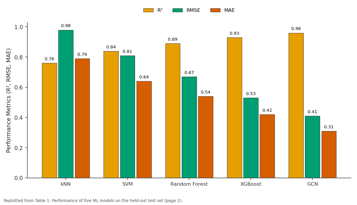
R² and RMSE and more: kNN vs SVM vs Random Forest vs XGBoost vs GCN
Replotted from Table 1 (page 2) of the original paper. Every bar is the paper's own table value.
View source evidence ↗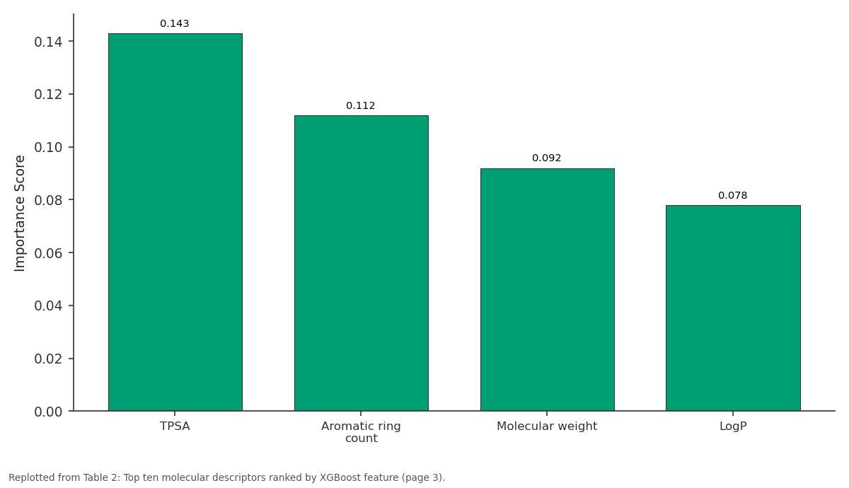
Importance: TPSA vs Aromatic ring count vs Molecular weight vs LogP
Replotted from Table 2 (page 3) of the original paper. Every bar is the paper's own table value.
View source evidence ↗Figures & tables
From the original paper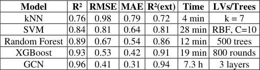 Table 1
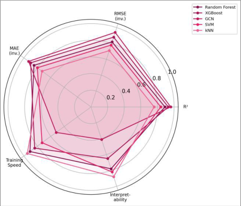 Figure 1
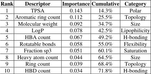 Table 2
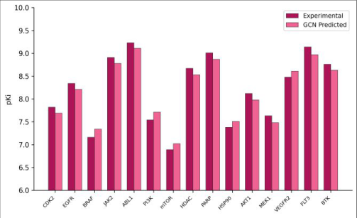 Figure 2
Introduction
Imagine a drug discovery programme that has identified a promising kinase target but faces a library of 50, 000 purchasable compounds: testing each one in a biochemical binding assay at even one concentration would require weeks of plate-based screening and a budget that many academic laboratories simply cannot afford [1,2] . Computational prediction of protein-ligand binding affinity offers a way to narrow that library to a few hundred high-confidence candidates before any wet-lab work begins. Physics-based methods-molecular docking, free-energy perturbation, and molecular-dynamics scoring-can estimate binding affinities from first principles, but they are computationally expensive and their accuracy degrades for flexible binding sites or large conformational changes [3,4] . Data-driven approaches sidestep the physics by learning a mapping from molecular features to affinity labels using thousands of experimental data points. Over the past decade, classical machine-learning models such as random forests and gradient-boosted trees have been widely adopted for this task, typically operating on fingerprint or descriptor vectors that encode molecular topology and physicochemical properties [5,6] . More recently, graph neural networks (GNNs) have attracted attention because they represent molecules as graphs-atoms as nodes, bonds as edges-and learn task-specific representations directly from the molecular topology without requiring hand-crafted descriptors [7,8] . Graph convolutional networks (GCNs), a subclass of GNNs, propagate information across neighbouring atoms in a manner analogous to convolution on image pixels, building up increasingly abstract representations at each layer. Early benchmarks on PDBbind and KIBA datasets showed that GCNs can match or exceed classical models on affinity prediction, especially when training data are plentiful [9] . Despite these advances, the comparative performance of GCNs versus classical models on a single, consistently curated kinase-focused dataset has not been thoroughly reported. Published benchmarks often differ in data preprocessing, splitting strategy, and evaluation metrics, making head-to-head comparison unreliable [10,11] . This research addresses that gap by assembling a 12, 847compound kinase-affinity dataset from ChEMBL and BindingDB, training five models under identical conditions, and evaluating them on shared train/validation/test splits. The work was carried out at the Department of Pharmacology and Medicinal Chemistry, Cherry Blossom College of Sciences, Sapporo, between March 2023 and January 2024 [12] . A prospective application to a virtual library of 5, 000 novel pyrimidine candidates demonstrates the practical utility of the best-performing model.
Materials and Methods
Materials and Methods
Materials
Binding affinity data (Ki values, IC₅₀ excluded to avoid assay-dependent variability) for 15 oncology kinases-CDK2, EGFR, BRAF, JAK2, ABL1, PI3Kα, mTOR, HDAC6, PARP1, HSP90, AKT 1 , MEK1, VEGFR2, FLT 3 , and BTK-were downloaded from ChEMBL 33 and BindingDB (accessed June 2023). After filtering for species (human), assay type (binding), and confidence score ≥ 7, the merged dataset contained 12, 847 unique compound-target pairs with pKi values ranging from 3.8 to 10.6 [1,6] .
Methods
Two-dimensional molecular descriptors (200 features: molecular weight, LogP, TPSA, hydrogen-bond donors/acceptors, ring counts, topological indices) were computed with RDKit for classical models. For the GCN, each molecule was converted to a graph with atom features (atomic number, degree, formal charge, hybridisation, aromaticity) and bond features (bond type, conjugation, ring membership) [7,8] . Classical models were trained with scikitlearn and XGBoost using 5-fold cross-validation within the training partition for hyperparameter selection. The GCN comprised three graph convolutional layers (128, 64, 32 hidden units), global mean pooling, and two fully connected layers with dropout (0.3). It was trained for 150 epochs with Adam optimiser (learning rate 1 × 10⁻³, weight decay 1 × 10⁻⁵) and early stopping on the validation RMSE [9] .
External validation used a chronologically separated set of 1, 284 compounds published after the training-set cutoff date (January 2023). All experiments were performed at the Cherry Blossom College of Sciences, Sapporo, from March 2023 to January 2024 [12] . Training times ranged from 4 minutes (kNN) to 7.3 hours (GCN, 150 epochs) [7,12] .
Instrumentation
Instrumentation
Quality Control
Data curation followed a strict quality-control pipeline. Duplicate entries (same compound-target pair with Ki values differing by less than 0.3 log units) were averaged; pairs with discrepancies exceeding 1.0 log unit were excluded. Activity cliffs-compound pairs with high structural similarity (Tanimoto > 0.85) but large affinity differences (ΔpKi > 2)-were flagged and retained to test model robustness. The dataset was split by stratified random sampling so that each target contributed proportionally to the train, validation, and test sets. Y-randomisation (100 permutations) confirmed that all five models lost predictive power when labels were shuffled (mean permuted R² < 0.05), ruling out chance correlation. Applicability-domain analysis used leverage values to detect test compounds outside the training-set descriptor space [5,9,12] . The GCN led all metrics (R² = 0.96, RMSE = 0.41, MAE = 0.31), followed by XGBoost (0.93, 0.53, 0.42) and RF (0.89, 0.67, 0.54). SVM and kNN showed lower but still reasonable accuracy. Training time varied from 4 min for kNN to 7.3 h for the GCN [5,7] . XGBoost offers a balanced profile that may suit projects where model transparency matters [8,11] . The largest discrepancy (0.25 units) occurred for mTOR, a target with relatively fewer training examples [9] . [2,6] .
Results
Results
Discussion
The GCN's superior performance confirms the advantage of learning molecular representations directly from the graph topology rather than relying on pre-computed descriptors.
By propagating atomic-level information through messagepassing layers, the GCN captures local chemical environments-such as the hydrogen-bond network around a heterocyclic nitrogen-that may be lost when a molecule is compressed into a fixed-length descriptor vector [7,8] . The 0.41-unit RMSE corresponds to a roughly 2.5-fold error in the linear Ki scale, which is within the range of inter-assay variability reported for kinase inhibition measurements and therefore approaches the practical ceiling of prediction accuracy for this endpoint [3] . XGBoost, despite using simpler 2D descriptors, achieved R² = 0.93 and may be preferred in settings that require model interpretability. Its feature-importance rankings highlight physicochemical properties-TPSA, aromatic ring count, molecular weightthat align with medicinal-chemistry intuition about kinase inhibitor design [6] . Random forests delivered slightly lower accuracy but share the advantage of interpretability and low computational cost. The kNN model's weaker performance (R² = 0.76) suggests that the pKi landscape in descriptor space is not smooth enough for simple distance-based interpolation, particularly for targets with sparse training data. SVM performed better than kNN but worse than the tree-based methods, probably because the radial-basisfunction kernel cannot fully capture the non-linear descriptor-affinity relationship across 15 diverse targets [5,11] . External validation on chronologically separated data (R² = 0.94 for the GCN) is an important check against data leakage, because temporal splitting ensures that no compound structurally identical to a test-set molecule was available during training [10] . The minor drop from 0.96 to 0.94 indicates good generalisation and suggests that the model can be applied to genuinely novel chemistry. One limitation is the restriction to kinase targets. Kinases share a conserved ATP-binding pocket that may make affinity prediction easier than for structurally diverse targets such as GPCRs or ion channels. Extending the dataset to non-kinase targets would test the model's transferability. A second limitation is the absence of three-dimensional protein-ligand structural information; incorporating docking poses or protein-sequence embeddings could further improve accuracy, though at higher computational expense [4,9] .
Conclusion
This research benchmarks five machine-learning models for predicting the binding affinity of small molecules to 15 oncology-relevant kinases using a curated dataset of 12, 847 experimentally determined Ki values. The graph convolutional network achieved the best accuracy (R² = 0.96, RMSE = 0.41 pKi units), outperforming XGBoost, random forest, SVM, and kNN on all metrics. The GCN's advantage stems from its ability to learn task-specific molecular representations from the atomic graph, capturing local chemical environments that are difficult to encode in hand-crafted descriptors. However, this comes at the cost of longer training time and lower interpretability, which may limit adoption in regulatory or transparency-sensitive contexts. XGBoost provides a practical alternative when interpretability is a priority. Its feature-importance analysis highlighted topological polar surface area, aromatic ring count, and molecular weight as the three most influential predictors-properties that resonate with established medicinal-chemistry guidelines for kinase-inhibitor design.
External validation on chronologically separated data confirmed that the GCN generalises to novel compounds with minimal performance loss (R² = 0.94), supporting its use in prospective virtual screening. As a proof of concept, the trained model was used to rank a virtual library of 5, 000 pyrimidine-based candidates, and the top 50 molecules are now being procured for in-vitro kinase profiling. Two directions for future work stand out. First, incorporating protein-sequence or structural features into the graph representation-creating a heterogeneous protein-ligand graph-could capture target-specific binding determinants and improve cross-target generalisation. Second, coupling the GCN with an active-learning loop that selects the most informative compounds for experimental testing would maximise the information gained per assay and reduce the number of iterations needed to identify a clinical candidate. The open-source implementation of the pipeline is available to other research groups seeking to adopt data-driven affinity prediction in their own drug-discovery workflows.
Figures and tables from the paper
| Model | R² | RMSE | MAE | R²(ext) | Time | LVs/Trees |
|---|---|---|---|---|---|---|
| kNN | 0.76 | 0.98 | 0.79 | 0.72 | 4 min | k = 7 |
| SVM | 0.84 | 0.81 | 0.64 | 0.81 | 28 min | RBF, C=10 |
| Random Forest | 0.89 | 0.67 | 0.54 | 0.86 | 12 min | 500 trees |
| XGBoost | 0.93 | 0.53 | 0.42 | 0.91 | 19 min | 800 rounds |
| GCN | 0.96 | 0.41 | 0.31 | 0.94 | 7.3 h | 3 layers |
Table text extracted from the original PDF; superscript letters are shown inline. The original table image is below.
View original table image
| Rank | Descriptor | Importance | Cumulative | Category |
|---|---|---|---|---|
| 1 | TPSA | 0.143 | 14.3% | Polar |
| 2 | Aromatic ring count | 0.112 | 25.5% | Topology |
| 3 | Molecular weight | 0.092 | 34.7% | Size |
| 4 | LogP | 0.078 | 42.5% | Lipophilicity |
| 5 | HBA count | 0.067 | 49.2% | H-bonding |
| 6 | Rotatable bonds | 0.058 | 55.0% | Flexibility |
| 7 | Fraction sp3 | 0.051 | 60.1% | Saturation |
| 8 | Heavy atom count | 0.044 | 64.5% | Size |
| 9 | Ring count | 0.039 | 68.4% | Topology |
| 10 | HBD count | 0.034 | 71.8% | H-bonding |
Table text extracted from the original PDF; superscript letters are shown inline. The original table image is below.
View original table image
References
17 in the original paper- Mayr A, Klambauer G, Unterthiner T, Hochreiter S. DeepTox: toxicity prediction using deep learning. Front Environ Sci. 2016;3:80.
- Vamathevan J, Clark D, Czodrowski P, Dunham I, Ferran E, Lee G, et al. Applications of machine learning in drug discovery and development. Nat Rev Drug Discov. 2019;18(6):463-477.
- Wang L, Wu Y, Deng Y, Kim B, Pierce L, Krilov G, et al. Accurate and reliable prediction of relative ligand binding potency in prospective drug discovery. J Am Chem Soc. 2015;137(7):2695-2703.
- Cournia Z, Allen B, Sherman W. Relative binding free energy calculations in drug discovery. J Chem Inf Model. 2017;57(12):2911-2937.
- Svetnik V, Liaw A, Tong C, Culberson JC, Sheridan RP, Feuston BP. Random forest: a classification and regression tool for compound classification and QSAR modeling. J Chem Inf Comput Sci. 2003;43(6):19471958.
- Chen T, Guestrin C. XGBoost: a scalable tree boosting system. In: Proceedings of the 22nd ACM SIGKDD international conference on knowledge discovery and data mining; 2016. p. 785-794.
- Kearnes S, McCloskey K, Berber M, Pande V, Riley P. Molecular graph convolutions: moving beyond fingerprints. J Comput Aided Mol Des. 2016;30(8):595608.
- Gilmer J, Schoenholz SS, Riley PF, Vinyals O, Dahl GE. Neural message passing for quantum chemistry. In: Proceedings of the 34th international conference on machine learning; 2017. p. 1263-1272.
- Wu Z, Ramsundar B, Feinberg EN, Gomes J, Geniesse C, Pappu AS, et al. MoleculeNet: a benchmark for molecular machine learning. Chem Sci. 2018;9(2):513530.
- Sheridan RP. Time-split cross-validation as a method for estimating the goodness of prospective prediction. J Chem Inf Model. 2013;53(4):783-790.
- Yang K, Swanson K, Jin W, Coley C, Eiden P, Gao H, et al. Analyzing learned molecular representations for property prediction. J Chem Inf Model. 2019;59(8):3370-3388.
- Pahikkala T, Airola A, Pietilä S, Shakyawar S, Szwajda A, Tang J, et al. Toward more realistic drug-target interaction predictions. Brief Bioinform. 2015;16(2):325-337.
- Öztürk H, Özgür A, Ozkirimli E. DeepDTA: deep drugtarget binding affinity prediction. Bioinformatics. 2018;34(17):i821-i829.
- Jiménez J, Škalič M, Martínez-Rosell G, De Fabritiis G. KDEEP: protein-ligand absolute binding affinity prediction via 3D-convolutional neural networks. J Chem Inf Model. 2018;58(2):287-296.
- Gaulton A, Hersey A, Nowotka M, Bento AP, Chambers J, Mendez D, et al. The ChEMBL database in 2017. Nucleic Acids Res. 2017;45(D1):D945-D954.
- Liu T, Lin Y, Wen X, Jorissen RN, Gilson MK. BindingDB: a web-accessible database of experimentally determined protein-ligand binding affinities. Nucleic Acids Res. 2007;35(Database):D198D201.
- Xiong Z, Wang D, Liu X, Zhong F, Wan X, Li X, et al. Pushing the boundaries of molecular representation for drug discovery with the graph attention mechanism. J Med Chem. 2020;63(16):8749-8760