
Research article · 2026 · Full text
International Journal of Geography Geology and EnvironmentKappa Coefficient accuracy estimation for assessing the major components of Mudbank formation through the temporal scale (24 years) of the Subarnarekha river estuary zone, Odisha, India.
Volume 8(1) · Pages 01–10 · DOI: 10.22271/27067483.2026.v8.i1a.464 ↗
Research areasGroundwater and Watershed AnalysisRemote-Sensing Image ClassificationCoastal wetland ecosystem dynamics
Abstract
Author-writtenRemote sensing is an important tool and technique for the best assessment of LULC map preparation and satellite image classification. This study emphasizes the classification of LULC of the adjacent lower zone area of the Subarnarekha River. To complete this study, ten such parameters have been considered, like Water-Body, Vegetation, Settlement, agricultural land area, Point Bar, Sand Bar, Sand Bank, Sand Dunes, Fishery Zone, and Mud-Bank Area at estuarine part of this river. Availability of Landsat images six specific years are sampled like 1998, 2004,2009,2014,2018 and 2022 respectively. The several factors have been consider including availability of quality Landsat imagery data through precise classification steps and users experience and expertise of the procedures. The objective of this study has been completed using the geospatial techniques like RS and GIS applications, which have compiled distinct two sections. First phase is containing Land-use and Land-cover (LULC) classification and, second phase is containing accuracy assessment of considered parameters. The Non-parametric Kappa coefficient Khat Statistic rule has applied for esteemed supervised classification with Kappa coefficient scale. The study had an overall classification accuracy of 86.75% and Kappa coefficient (K) of 0.911, 0.908, 0.719, 0.803, 0.858, and 0.886 following the considered study year. Overall accuracy through Khat Statistic reveals that vegetation, settlement, agricultural land, fishery and mud-bank are dominant parameters for the considered random samples. The revealed results are considerable and helpful for sustainable plan in future for this area.
Summary
Source-checkedPlain-language reading of the full paper, prepared with AI and checked against the text. Each point links to the authors' own words.
Why it matters
- Land use and land cover (LULC) analysis is a critical tool for understanding the geomorphological characteristics of a specific geographical area. View evidence ↗
- LULC changes are driven by both natural processes and human interference, such as demographic pressure and development activities. View evidence ↗
- Remote sensing provides an effective technique for preparing LULC maps and classifying satellite imagery. View evidence ↗
The question
- The study aims to classify the land use and land cover of the lower zone area of the Subarnarekha River. View evidence ↗
What they did
- The research focused on a study area totaling 467 square kilometers. View evidence ↗
- The analysis tracked ten geomorphological parameters, including water bodies, vegetation, settlements, agricultural land, and various sand and mud formations. View evidence ↗
- The supervised classification process utilized 40 identified training sites across the considered parameters. View evidence ↗
- The study used the non-parametric Kappa coefficient (Khat Statistic) to assess the accuracy of the supervised classification. View evidence ↗
What they found
- The overall classification accuracy for the study was 86.75%. View evidence ↗
- Overall accuracy fluctuated over the study period, with the highest accuracy of 93% in 1999 and the lowest of 75% in 2009. View evidence ↗
- Vegetation, settlement, agricultural land, fishery, and mud-banks were identified as the dominant parameters in the sampled areas. View evidence ↗
- The highest commission errors were observed in the vegetation, settlement, agriculture, and mud-bank categories. View evidence ↗
What it means
- The authors conclude that the Kappa coefficient is a valuable tool for supervised classification across different spatial resolutions. View evidence ↗
- The findings are considered useful for the future sustainable planning of the Subarnarekha river estuary zone. View evidence ↗
Visual summary
2 visualsIllustrations explain the paper; charts are replotted from the paper's own table values.
LULC Analysis Workflow
AI-generated conceptual illustration (Subarnarekha river estuary zone with mudbanks and satellite imagery). It explains the idea and does not show study data.
View source evidence ↗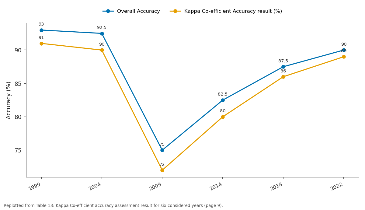
Overall Accuracy and Kappa Co-efficient Accuracy result (%): 1999 vs 2004 vs 2009 vs 2014 vs 2018
Replotted from Table 13 (page 9) of the original paper. Every bar is the paper's own table value.
View source evidence ↗Figures & tables
From the original paper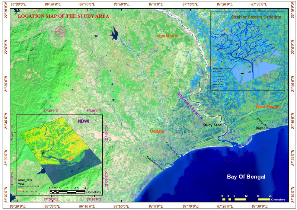 Figure 1
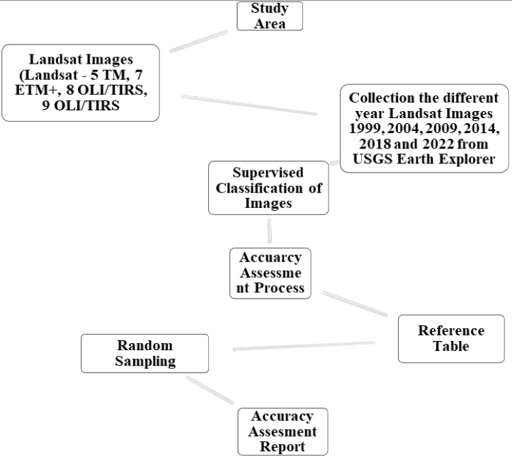 Figure 2
 Table 1
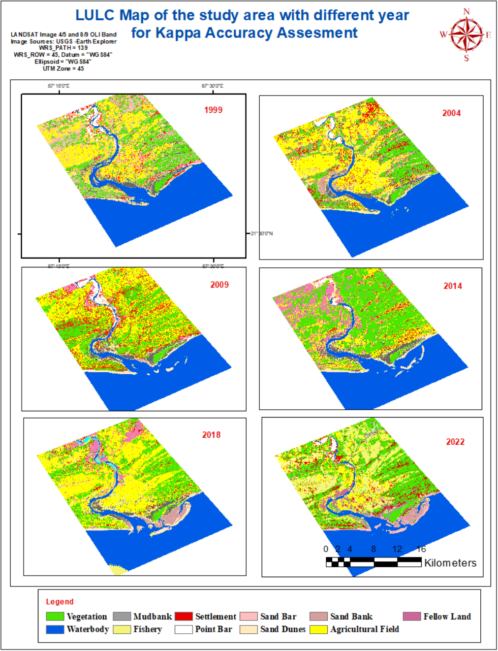 Figure 2
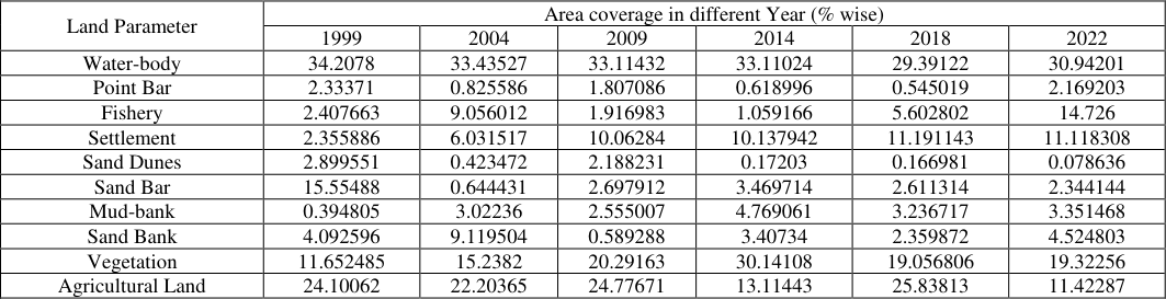 Table 2
 Table 3
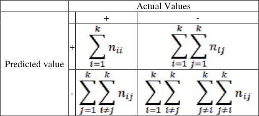 Table 4
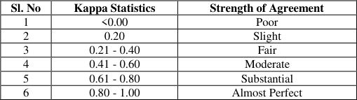 Table 5
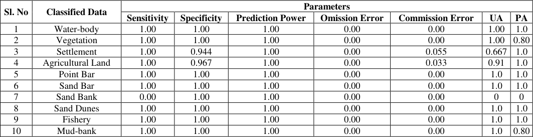 Table 6
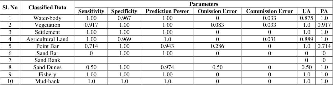 Table 7
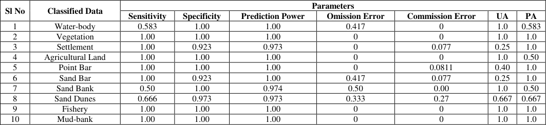 Table 8
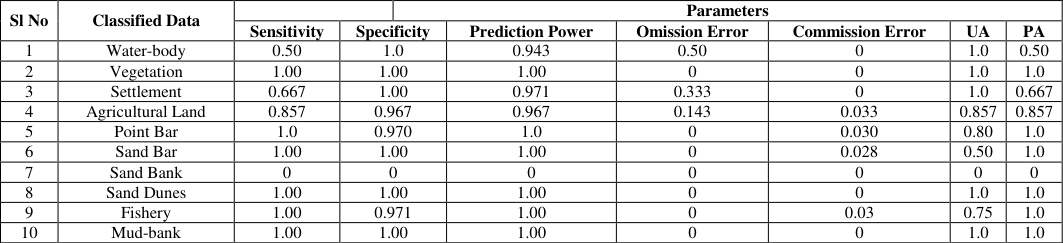 Table 9
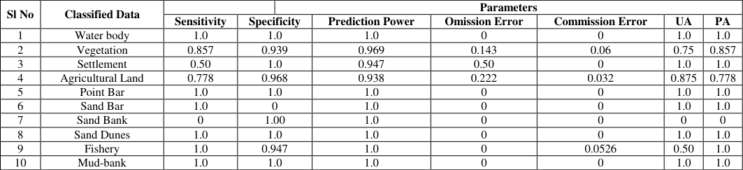 Table 10
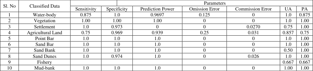 Table 11
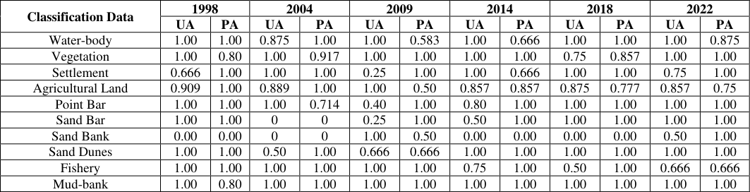 Table 12
 Table 13
 Table 14
Introduction
Baulies (1997) [2] suggested that the land use and land cover changes dynamically due to pressure of demographic activities and related human development activities. So that, land use and land cover change definitely be the result of natural process and human interference (Turner et al., 1994, Tucker et al., 1991) [21,22] . Moreover, the technological advancement and expending population have put an increasing trend of pressure on localized scarce resources and have compiled a variety of complex land use dilemmas that affect individually or wholly at all levels of entire society (Sommers, 1981) [18] . Application of Land use and land cover (LULC) analysis is the very important step for analysing the geomorphological characteristics of any geographical space. In every LULC studies are very crucial and effective for the estimating of physical characteristics of any place. Considering the selected parameters, this calculation has played a vital role for environmental planning and management. Many researchers tried to estimate the actual position of the geomorphological characteristics through the model building techniques in recent time. The LULC study is used for the input data of model which runs in present time for calculating the changing nature of physical features. Moreover, LULC is the outcome of interdisciplinary considerable parameters, such as geo-morphological, geo-biophysical, socio-economic, systems behaviours and interaction with other related things. The updated application of hybrid classification combines the unsupervised and supervised techniques of LULC classification in two stages. An unsupervised method is used to achieve a number of naturally cloven categories in the first stage.
After the segregation of each category, the identification of considered parameters is confirmed through the aid of proper reference image. After that the training data has been generated with the help of these prior natural data. However, the selected classes that are ambiguous as well as may represent more than one LULC class or category can be discarded. This step helps to frame up a far crisper training dataset as an input for the supervised category. Sader, Ahi and Liou (1995) [19] have done a comparative analysis for the accuracy of various classification approaches and have revealed that the classification through the hybrid method supersedes the unsupervised and supervised methods by using the case study of Acadian wetlands. Similarly, hybrid classification of an unsupervised and supervised classification approaches are more applicable for the classification of complex ecosystem components (Ozesmi and Bauer, 2002) [14] . The application of remote sensing track out the changes occurred in LULC where the use of multi-date images analysed. A proper monitoring process has run thoroughly when this multi date image classification run. During the analysis of multi-date imageries the differences occurring in LULC values between the acquisition dates if considered images that are mainly due to temporally various natural conditions and human actions. O.R. Abd El-Kawy et al., 2010, [15] ensuring that the prosperous use of satellite remote sensing for LULC change detection highly depends upon adequate understanding of considered land scape features, image system methodology used in relation to the aim of study. Accuracy assessment or validation of morphological change detection is a significant gradation in the processing of remote sensing data. That assessment emphasizes the information values of the resulting data to any user. Quantitative utilization of geodata is only possible when the quality of considered data is known. Finally overall accuracy has to be calculated as per compare with the classified pixel versus definite land cover conditions which has obtained from corresponding ground truth data. This application leads to two types of error corresponding to producers and User accuracy but all classified pixels are checked by the ground truth. So, real locational and physical changes should be prominent through this assessment (Congalton, R.G.1991, Campbell, J.B. 2007, Jensen, J.R. 2005) [7,3,11] .
Study area
The Subarnarekha estuary is situated at the Balasore district of Odisha state and its mouth width is 4. 10 This study has been concentrated on supervised classification of considered images. This classification is most suitable for comparison of LULC classification through the spectral signatures of known and unknown categories (Eastman, J.R. 2003) [7] . Many researchers believe that, supervised classification when image processing is effective for quantitative analysis of remote sensing data (Richards, J. and Jia, X. 2006) [16] . The supervised classification depends on training site data preparation along with LULC rectification, so we have executed the prior knowledge to utilize the supervised classification. As per suggestion of the renowned researchers it is necessary to collect spectral signatures from considered training sites during the execution of supervised classification which are used to "train" the classification algorithm (Chen and Stow, 2002; Jusoff et al., 2009) [5,12] .
1) Demarcation of training sites
After the confirmation of selected components area that will be used
2) Extraction of spectral signature
All the considered classes have been separated by selecting the spectral signatures of each class from different image sites, using the seed properties method through ERDAS imagine. The output from the seed properties was manually corrected by ARC GIS 10.8 along with 30 meter spatial resolution. Moreover, the image was improved and enhanced using digital image enhancement processing techniques to confirm each LULC class before interpretation. Comparative area coverage in percentage of considered six years extracted result is given in Table-2. In this study a supervised classification using maximum likelihood was applied based on the spectral differences between different classes. These differences were used to subdivide the LULC of the LZRB into separate classes. Prior knowledge is utilized to execute supervised classification, depending on previously collected training sites from certain areas of known LULC. In order to execute a supervised classification, it is necessary to collect spectral signatures from training areas, which are then used to "train" the classification algorithm (Chen and Stow 2002; Jusoff et al. 2009) [5,12] . Several training sites were collected from different places of the study area depending on the collected ground control points, field observations and the auxiliary data. Training sites for each LULC class were collected by selecting many training sites for the same class considering their spatial distribution. Based on the statistics of these training sites, each pixel in the classified image of the LULC map was then assigned to these training sites. The LULC map for the LZRB was generated based on the pixel-by-pixel supervised classification using Landsat 8 OLI images from September 2014. Classes have been separated by selecting the spectral signatures of each class from different image sites, using the seed properties method that is provided in ERDAS Imagine V.11 software. The results were manually corrected by ArcGIS, using mainly OLI-8 images of 30-meter spatial resolution. The image was improved and enhanced using digital image enhancement processing techniques to highlight some LULC classes before interpretation. Image enhancement processes alter the impression of the image on the viewer. In ERDAS software, different enhancement techniques are available: contrast enhancement, linear and nonlinear contrast stretching, density slicing, Gaussian stretching and so forth. Because the enhancement distorts digital pixel values, supervised classification was carried out on the original images.
3) Accuracy assessment
Accuracy assessment is a robust technique in scientific field field to detect the rectification of satellite data in recent time. Different scientific community have uses these data through the software application of image processing. This analysis provides faster and more powerful result in remote sensing field. The result obtained from the satellite image processing is always accompanied with certain error probability during the analysis. Accuracy assessment is considered to be the metering of vicinity of the given results which values accepted as true. For estimation to evaluate thematic maps produced from raster images the testing of accuracy of the classification and evaluating the agreement of the output map for the particular purpose is the main approach (Foody G.M, 2008) [8] . This assessment is emphasis on and comparing the classification results with known information. The minimum level of interpretation accuracy for the identification of considered LULC categories from remote sensor data should be at least 85 % in average (Wright and Morrice 1997; Anderson et al. 1976). [23,1] Through the application of accuracy assessment the target value achieve as correct at 85% and typically should be standard for image classification. The attractiveness of the target values specified its accuracy as per its comparable factors (Foody, 2002) [9] . There are several factors which can directly affect the accuracy values for indicating the characteristics of the satellite data, such as extension of the study area and considered LULC classes. Thematic maps extracted from the remote sensing data always follow a statistically intense accuracy assessment before being used for scientific investigations (Stehman and Czaplewski 1998) [17] . In this study, accuracy has been evaluated with an error matrix which is popularly known as confusion matrix. An error of confusion matrix is the most common steps used for calculating the accuracy of any thematic maps derived from multispectral imagery (Smits et al. 1999; Congalton and Green 2002; Liu et al. 2007) [20,6,13] . The estimated error matrix highlights the results from the comparison of reference class corresponding to the LULC categories with the real results.
Confusion Matrix:
The confusion matrix is considered as the standard step to estimate the performance of collected data. This includes sensitivity and specificity, commission and omission error and positive and negative predictive power (Fielding and Bell, 1997) [10] . Computation is based on a "Confusion Matrix", reflecting the four possible ways, as follows:
Actual Values
Predicted value β = number of times a point was classified as X when it was observed to be X. γ = Number of times a point was not classified as X when it was observed to be X. α = Number of times a point was classified as X when it was observed to be not X.
as X when it was not observed to be X Therefore, Sensitivity = α / (α + γ), it is equivalent to Producer's Accuracy.
Specificity = ∆ / (β + ∆)
False Positive Rate (Commission Error) = β / (β + ∆) = (1 -Specificity)
False Negative Rate (Omission Error) = γ / (α + γ) = (1 -Sensitivity)
Positive Predictive Power = α / (α + β) (Equivalent to User's Accuracy)
Negative Predictive Power = ∆ / (∆ + γ) Therefore, ten categories of error matrix have been calculated for this study (Table -3).
Now weighted average model statistics may be generated by combining those metrics over all classification as per following equations (Table -4).
Where, ∑_(i = 1)^k n_{ii} = Sum of diagonal elements.
∑_(i = 1)^k ∑_(j=1)^k n_{ij} = Sum of non-diagonal elements.
∑_(j = 1)^k ∑_(i≠j)^k n_{ij} = Sum of non-diagonal elements.
∑_(i = 1)^k ∑_(i≠j)^k ∑_(j≠i)^k n_{ij} = Sum of nonrow/column elements.
KAPPA co-efficient
Moreover KAPPA statistics has been applied for accuracy assessment for this study. KAPPA analysis is a discrete multivariate technique which used in accuracy assessment. KAPPA analysis yields a Khat statistic (an estimate of KAPPA) that is a measure of agreement or accuracy. The Khat statistic is computed as:
Where: r = Number of rows and columns in the error matrix. N = Total number of observations. xᵢᵢ = Observation in row i and column i. xᵢ₊ = Marginal total of row i, and x₊ᵢ = Marginal total of column i.
The Kappa co-efficient equal to 1 means perfect agreement where as calculated value close to zero means the agreement is not better than would be expected by chance. The categorization of Kappa statistic is widely referenced which is given in Table-5.
Result and Discussion
Following the step-wise assessment under supervised classification, the considered area has been derived such fruitful results for leading explanation. In this paper we have tried to understand the results of comparative analysis of LULC along with accuracy assessment through remote sensing application. Using the formulae furnished earlier, ten parameters were evaluated and analysed. After the allocation of each considered parameters, their area has been confirmed taking into account the pixel count in respect of total area. The considered parameters are water-body, vegetation, settlement, agricultural land, point bar, sand bar, sand bank, sand dunes, fisheries area, and mud-bank respectively. During the step-wise supervised classification, 40 training sites have been considered for six year-wise images as 1998, 2004, 2009, 2014, 2018 and 2022 respectively. The aims of accuracy assessment were to quantitatively assess how effectively the pixels were sampled for the correct land-use and land-cover classes. Moreover the steps emphasis on accuracy assessment for pixel selection was on area that could be finally identified on considered land-sat high resolution image, Google Earth and Google Map respectively. The accuracy assessment cell array reference columns were computed accordingly on the best guess of each sampled reference points. Depends on the confusion matrix (error matrix), of LULC classification, the image pixel have been assigned into the ground truth. This computation helps to understand the proper results for true accuracy for both considered dataset. As per the results given in
Conclusion
Image classification is a robust technical method for Landuse and land cover analysis using satellite images. Many researchers widely adopted this method during last recent decades for analysing the reliability of ground truth with the help of corresponding images. This study emphasizes adjacent river bank land use and land cover classification at lower part of Subarnarekha River. LULC maps production at considered kappa co-efficient scale for different yearly images have been completed in this study. Advancement of supervised classification through pixel to pixel rectification has revealed the accuracy results for considered parameters in different years. After the supervised classification applying non-parametric rules, the images were classified into six categorical classes as per their Kappa co-efficient accuracy magnitude (Table -13). The overall weighted average value is also estimated for the concluding remark which is given in Table-14. The result indicates less amount of error in respect of User's accuracy as well as Producer's accuracy and some dominant considered components are vegetation, settlement, agriculture, fishery and mud-bank coverage. The considered kappa coefficient is a worthy technique as substantial and hence the classified images to be competent for further study.
Figures and tables from the paper
| Sl. No | Satellite | Sensor ID | WRS Path | WRS Row | Date of Acquisition | Grid cell size (m) |
|---|---|---|---|---|---|---|
| 1 | Landsat-7 ETM | LE71390451999342SGS01 | 139 | 045 | 1999-12-08 | 30 |
| 2 | Landsat-5 TM | LT51390452004364BKT00 | 139 | 045 | 2004-12-29 | |
| 3 | Landsat-5 TM | LT51390452009297KHC00 | 139 | 045 | 2009-10-24 | |
| 4 | Landsat-8 OLI/TIRS | LC81390452014087LGN01 | 139 | 045 | 2014-03-28 | |
| 5 | Landsat-8 OLI/TIRS | LC81390452018322LGN00 | 139 | 045 | 2018-11-18 | |
| 6 | Landsat-9 OLI/TIRS | LC91390452022037LGN00 | 139 | 045 | 2022-02-06 |
Table text extracted from the original PDF; superscript letters are shown inline. The original table image is below.
View original table image
| Land Parameter | Area coverage in different Year (% wise) | — | — | — | — | — |
|---|---|---|---|---|---|---|
| 1999 | 2004 | 2009 | 2014 | 2018 | 2022 | |
| Water-body | 34.2078 | 33.43527 | 33.11432 | 33.11024 | 29.39122 | 30.94201 |
| Point Bar | 2.33371 | 0.825586 | 1.807086 | 0.618996 | 0.545019 | 2.169203 |
| Fishery | 2.407663 | 9.056012 | 1.916983 | 1.059166 | 5.602802 | 14.726 |
| Settlement | 2.355886 | 6.031517 | 10.06284 | 10.137942 | 11.191143 | 11.118308 |
| Sand Dunes | 2.899551 | 0.423472 | 2.188231 | 0.17203 | 0.166981 | 0.078636 |
| Sand Bar | 15.55488 | 0.644431 | 2.697912 | 3.469714 | 2.611314 | 2.344144 |
| Mud-bank | 0.394805 | 3.02236 | 2.555007 | 4.769061 | 3.236717 | 3.351468 |
| Sand Bank | 4.092596 | 9.119504 | 0.589288 | 3.40734 | 2.359872 | 4.524803 |
| Vegetation | 11.652485 | 15.2382 | 20.29163 | 30.14108 | 19.056806 | 19.32256 |
| Agricultural Land | 24.10062 | 22.20365 | 24.77671 | 13.11443 | 25.83813 | 11.42287 |
Table text extracted from the original PDF; superscript letters are shown inline. The original table image is below.
View original table image
| — | Actual Values | — | — |
|---|---|---|---|
| Predicted value | + | - | |
| + | α | β | |
| - | ϒ | Δ |
Table text extracted from the original PDF; superscript letters are shown inline. The original table image is below.
View original table image
| — | Actual Values | — | — |
|---|---|---|---|
| Predicted value | + | - | |
| + | |||
| - |
Table text extracted from the original PDF; superscript letters are shown inline. The original table image is below.
View original table image
| Sl. No | Kappa Statistics | Strength of Agreement |
|---|---|---|
| 1 | <0.00 | Poor |
| 2 | 0.20 | Slight |
| 3 | 0.21 - 0.40 | Fair |
| 4 | 0.41 - 0.60 | Moderate |
| 5 | 0.61 - 0.80 | Substantial |
| 6 | 0.80 - 1.00 | Almost Perfect |
Table text extracted from the original PDF; superscript letters are shown inline. The original table image is below.
View original table image
| Sl. No | Classified Data | Parameters | — | — | — | — | — | — |
|---|---|---|---|---|---|---|---|---|
| Sensitivity | Specificity | Prediction Power | Omission Error | Commission Error | UA | PA | ||
| 1 | Water-body | 1.00 | 1.00 | 1.00 | 0.00 | 0.00 | 1.00 | 1.0 |
| 2 | Vegetation | 1.00 | 1.00 | 1.00 | 0.00 | 0.00 | 1.00 | 0.80 |
| 3 | Settlement | 1.00 | 0.944 | 1.00 | 0.00 | 0.055 | 0.667 | 1.0 |
| 4 | Agricultural Land | 1.00 | 0.967 | 1.00 | 0.00 | 0.033 | 0.91 | 1.0 |
| 5 | Point Bar | 1.00 | 1.00 | 1.00 | 0.00 | 0.00 | 1.0 | 1.0 |
| 6 | Sand Bar | 1.00 | 1.00 | 1.00 | 0.00 | 0.00 | 1.0 | 1.0 |
| 7 | Sand Bank | 0.00 | 1.00 | 1.00 | 0.00 | 0.00 | 0 | 0 |
| 8 | Sand Dunes | 1.00 | 1.00 | 1.00 | 0.00 | 0.00 | 1.0 | 1.0 |
| 9 | Fishery | 1.00 | 1.00 | 1.00 | 0.00 | 0.00 | 1.0 | 1.0 |
| 10 | Mud-bank | 1.00 | 1.00 | 1.00 | 0.00 | 0.00 | 1.0 | 0.80 |
Table text extracted from the original PDF; superscript letters are shown inline. The original table image is below.
View original table image
| Sl. No | Classified Data | Parameters | — | — | — | — | — | — |
|---|---|---|---|---|---|---|---|---|
| Sensitivity | Specificity | Prediction Power | Omission Error | Commission Error | UA | PA | ||
| 1 | Water-body | 1.00 | 0.967 | 1.00 | 0 | 0.033 | 0.875 | 1.0 |
| 2 | Vegetation | 0.917 | 1.00 | 1.00 | 0.083 | 0.033 | 1.0 | 0.917 |
| 3 | Settlement | 1.00 | 1.00 | 1.00 | 0 | 0 | 1.0 | 1.0 |
| 4 | Agricultural Land | 1.00 | 0.969 | 1.0 | 0 | 0.031 | 0.889 | 1.0 |
| 5 | Point Bar | 0.714 | 1.00 | 0.943 | 0.286 | 0 | 1.0 | 0.714 |
| 6 | Sand Bar | 0 | 1.00 | 1.00 | 0 | 0 | 0 | 0 |
| 7 | Sand Bank | 0 | 0 | |||||
| 8 | Sand Dunes | 0.50 | 1.00 | 0.974 | 0.50 | 0 | 0.50 | 1.0 |
| 9 | Fishery | 1.00 | 1.00 | 1.00 | 0 | 0 | 1.0 | 1.0 |
| 10 | Mud-bank | 1.0 | 1.0 | 1.0 | 0 | 0 | 1.0 | 1.0 |
Table text extracted from the original PDF; superscript letters are shown inline. The original table image is below.
View original table image
| Sl No | Classified Data | Parameters | — | — | — | — | — | — |
|---|---|---|---|---|---|---|---|---|
| Sensitivity | Specificity | Prediction Power | Omission Error | Commission Error | UA | PA | ||
| 1 | Water-body | 0.583 | 1.00 | 1.00 | 0.417 | 0 | 1.0 | 0.583 |
| 2 | Vegetation | 1.00 | 1.00 | 1.00 | 0 | 0 | 1.0 | 1.0 |
| 3 | Settlement | 1.00 | 0.923 | 0.973 | 0 | 0.077 | 0.25 | 1.0 |
| 4 | Agricultural Land | 1.00 | 1.00 | 1.00 | 0 | 0 | 1.0 | 0.50 |
| 5 | Point Bar | 1.00 | 1.00 | 1.00 | 0 | 0.0811 | 0.40 | 1.0 |
| 6 | Sand Bar | 1.00 | 0.923 | 1.00 | 0.417 | 0.077 | 0.25 | 1.0 |
| 7 | Sand Bank | 0.50 | 1.00 | 0.974 | 0.50 | 0.00 | 1.0 | 0.50 |
| 8 | Sand Dunes | 0.666 | 0.973 | 0.973 | 0.333 | 0.27 | 0.667 | 0.667 |
| 9 | Fishery | 1.00 | 1.00 | 1.00 | 0 | 0 | 1.0 | 1.0 |
| 10 | Mud-bank | 1.00 | 1.00 | 1.00 | 0 | 0 | 1.0 | 1.0 |
Table text extracted from the original PDF; superscript letters are shown inline. The original table image is below.
View original table image
| Sl No | Classified Data | — | — | Parameters | — | — | — | — | — |
|---|---|---|---|---|---|---|---|---|---|
| Sensitivity | Specificity | Prediction Power | Omission Error | Commission Error | UA | PA | |||
| 1 | Water-body | 0.50 | 1.0 | 0.943 | 0.50 | 0 | 1.0 | 0.50 | |
| 2 | Vegetation | 1.00 | 1.00 | 1.00 | 0 | 0 | 1.0 | 1.0 | |
| 3 | Settlement | 0.667 | 1.00 | 0.971 | 0.333 | 0 | 1.0 | 0.667 | |
| 4 | Agricultural Land | 0.857 | 0.967 | 0.967 | 0.143 | 0.033 | 0.857 | 0.857 | |
| 5 | Point Bar | 1.0 | 0.970 | 1.0 | 0 | 0.030 | 0.80 | 1.0 | |
| 6 | Sand Bar | 1.00 | 1.00 | 1.00 | 0 | 0.028 | 0.50 | 1.0 | |
| 7 | Sand Bank | 0 | 0 | 0 | 0 | 0 | 0 | 0 | |
| 8 | Sand Dunes | 1.00 | 1.00 | 1.00 | 0 | 0 | 1.0 | 1.0 | |
| 9 | Fishery | 1.00 | 0.971 | 1.00 | 0 | 0.03 | 0.75 | 1.0 | |
| 10 | Mud-bank | 1.00 | 1.00 | 1.00 | 0 | 0 | 1.0 | 1.0 |
Table text extracted from the original PDF; superscript letters are shown inline. The original table image is below.
View original table image
| Sl No | Classified Data | — | — | Parameters | — | — | — | — | — |
|---|---|---|---|---|---|---|---|---|---|
| Sensitivity | Specificity | Prediction Power | Omission Error | Commission Error | UA | PA | |||
| 1 | Water body | 1.0 | 1.0 | 1.0 | 0 | 0 | 1.0 | 1.0 | |
| 2 | Vegetation | 0.857 | 0.939 | 0.969 | 0.143 | 0.06 | 0.75 | 0.857 | |
| 3 | Settlement | 0.50 | 1.0 | 0.947 | 0.50 | 0 | 1.0 | 1.0 | |
| 4 | Agricultural Land | 0.778 | 0.968 | 0.938 | 0.222 | 0.032 | 0.875 | 0.778 | |
| 5 | Point Bar | 1.0 | 1.0 | 1.0 | 0 | 0 | 1.0 | 1.0 | |
| 6 | Sand Bar | 1.0 | 0 | 1.0 | 0 | 0 | 1.0 | 1.0 | |
| 7 | Sand Bank | 0 | 1.00 | 1.0 | 0 | 0 | 0 | 0 | |
| 8 | Sand Dunes | 1.0 | 1.0 | 1.0 | 0 | 0 | 1.0 | 1.0 | |
| 9 | Fishery | 1.0 | 0.947 | 1.0 | 0 | 0.0526 | 0.50 | 1.0 | |
| 10 | Mud-bank | 1.0 | 1.0 | 1.0 | 0 | 0 | 1.0 | 1.0 |
Table text extracted from the original PDF; superscript letters are shown inline. The original table image is below.
View original table image
| Sl. No | Classified Data | — | — | Parameters | — | — | — | — | — |
|---|---|---|---|---|---|---|---|---|---|
| Sensitivity | Specificity | Prediction Power | Omission Error | Commission Error | UA | PA | |||
| 1 | Water-body | 0.875 | 1.0 | 0.9697 | 0.125 | 0 | 1.0 | 0.875 | |
| 2 | Vegetation | 1.00 | 1.00 | 1.00 | 0 | 0 | 1.0 | 1.00 | |
| 3 | Settlement | 1.0 | 0.973 | 0 | 0 | 0.0270 | 0.75 | 1.00 | |
| 4 | Agricultural Land | 0.75 | 0.969 | 0.939 | 0.25 | 0.031 | 0.857 | 0.75 | |
| 5 | Point Bar | 1.0 | 1.0 | 1.0 | 0 | 0 | 1.0 | 1.00 | |
| 6 | Sand Bar | 1.0 | 1.0 | 1.0 | 0 | 0 | 1.0 | 1.00 | |
| 7 | Sand Bank | 1.0 | 1.0 | 1.0 | 0 | 0 | 0.50 | 1.00 | |
| 8 | Sand Dunes | 1.0 | 0.974 | 1.0 | 0 | 0.026 | 1.0 | 1.00 | |
| 9 | Fishery | 0.667 | 0.667 | ||||||
| 10 | Mud-bank | 1.0 | 1.0 | 1.0 | 0 | 0 | 1.00 | 1.00 |
Table text extracted from the original PDF; superscript letters are shown inline. The original table image is below.
View original table image
| Classification Data | 1998 | — | 2004 | — | 2009 | — | 2014 | — | 2018 | — | 2022 | — |
|---|---|---|---|---|---|---|---|---|---|---|---|---|
| UA | PA | UA | PA | UA | PA | UA | PA | UA | PA | UA | PA | |
| Water-body | 1.00 | 1.00 | 0.875 | 1.00 | 1.00 | 0.583 | 1.00 | 0.666 | 1.00 | 1.00 | 1.00 | 0.875 |
| Vegetation | 1.00 | 0.80 | 1.00 | 0.917 | 1.00 | 1.00 | 1.00 | 1.00 | 0.75 | 0.857 | 1.00 | 1.00 |
| Settlement | 0.666 | 1.00 | 1.00 | 1.00 | 0.25 | 1.00 | 1.00 | 0.666 | 1.00 | 1.00 | 0.75 | 1.00 |
| Agricultural Land | 0.909 | 1.00 | 0.889 | 1.00 | 1.00 | 0.50 | 0.857 | 0.857 | 0.875 | 0.777 | 0.857 | 0.75 |
| Point Bar | 1.00 | 1.00 | 1.00 | 0.714 | 0.40 | 1.00 | 0.80 | 1.00 | 1.00 | 1.00 | 1.00 | 1.00 |
| Sand Bar | 1.00 | 1.00 | 0 | 0 | 0.25 | 1.00 | 0.50 | 1.00 | 1.00 | 1.00 | 1.00 | 1.00 |
| Sand Bank | 0.00 | 0.00 | 0 | 0 | 1.00 | 0.50 | 0.00 | 0.00 | 0.00 | 0.00 | 0.50 | 1.00 |
| Sand Dunes | 1.00 | 1.00 | 0.50 | 1.00 | 0.666 | 0.666 | 1.00 | 1.00 | 1.00 | 1.00 | 1.00 | 1.00 |
| Fishery | 1.00 | 1.00 | 1.00 | 1.00 | 1.00 | 1.00 | 0.75 | 1.00 | 0.50 | 1.00 | 0.666 | 0.666 |
| Mud-bank | 1.00 | 0.80 | 1.00 | 1.00 | 1.00 | 1.00 | 1.00 | 1.00 | 1.00 | 1.00 | 1.00 | 1.00 |
Table text extracted from the original PDF; superscript letters are shown inline. The original table image is below.
View original table image
| Sl. No | Year | Overall Accuracy | Kappa Co-efficient Accuracy Result | Kappa Co-efficient Accuracy result (%) | Result |
|---|---|---|---|---|---|
| 1 | 1999 | 93 % | 0.911 | 91% | Almost Perfect |
| 2 | 2004 | 92.5 % | 0.908 | 90% | Almost Perfect |
| 3 | 2009 | 75 % | 0.719 | 72% | Substantial |
| 4 | 2014 | 82.5 % | 0.803 | 80% | Almost Perfect |
| 5 | 2018 | 87.5 % | 0.858 | 86% | Almost Perfect |
| 6 | 2022 | 90 % | 0.886 | 89% | Almost Perfect |
Table text extracted from the original PDF; superscript letters are shown inline. The original table image is below.
View original table image
| Parameter Type | 1998 | 2004 | 2009 | 2014 | 2018 | 2022 |
|---|---|---|---|---|---|---|
| Overall Weighted Average Sensitivity | 0.949 | 0.902 | 0.811 | 0.892 | 0.875 | 0.878 |
| Overall Weighted Average Specificity | 0.860 | 0.994 | 0.972 | 0.988 | 0.887 | 0.989 |
| Overall Weighted Average Omission Error | 0.0526 | 0.09756 | 0.1892 | 0.108 | 0.125 | 0.122 |
| Overall Weighted Average Commission Error | 0.0082 | 0.0057 | 0.028 | 0.012 | 0.0125 | 0.0084 |
Table text extracted from the original PDF; superscript letters are shown inline. The original table image is below.
View original table image
References
23 in the original paper- Anderson BJ, Hardy EE, Roach JT, Witmer RE. A land use and land cover classification system for use with remote sensor data. U.S. Geological Survey Professional Paper. 1976;964:1-41.
- Baulies X, Szejwach G, editors. Survey of needs, gaps and priorities on data for land use-land cover change research. LUCC Data Requirements Workshop; 1997;
- Campbell JB. Introduction to remote sensing. 4th ed. New York: The Guilford Press; 2007. p. 1-667.
- Congalton RG. A review of assessing the accuracy of classifications of remotely sensed data. Remote Sensing of Environment. 1991;37(1):35-46.
- Chen D, Stow D. The effect of training strategies on supervised classification at different spatial resolutions. Photogrammetric Engineering and Remote Sensing. 2002;68(11):1155-1162.
- Congalton RG, Green K. Assessing the accuracy of remotely sensed data: principles and practices. Boca Raton: Taylor & Francis; 2002. p. 1-137.
- Eastman JR. Guide to GIS and image processing. Vol. 14. Worcester: Clark University Manual; 2003. p. 239247.
- Foody GM. Harshness in image classification accuracy assessment. International Journal of Remote Sensing. 2008;29(11):3137-3158.
- Foody GM. Status of land cover classification accuracy assessment. Remote Sensing of Environment. 2002;80(1):185-201.
- Fielding AH, Bell JF. A review of methods for the assessment of prediction errors in conservation presence/absence models. Environmental Conservation. 1997;24(1):38-49.
- Jensen JR. Introductory digital image processing: a remote sensing perspective. 3rd ed. Upper Saddle River (NJ): Pearson Prentice Hall; 2005. p. 1-526.
- Jusoff K, Ismail MH, Ali NH. Spectral separability of tropical forest tree species using airborne hyperspectral imager. Journal of Environmental Science and Engineering. 2009;3(1):37-41.
- Liu C, Frazier P, Kumar L. Comparative assessment of the measures of thematic classification accuracy. Remote Sensing of Environment. 2007;107(4):606-616.
- Özemi SL, Bauer ME. Satellite remote sensing of wetlands. Wetlands Ecology and Management. 2002;10(5):381-402.
- Abd El-Kawy OR, Rod JK, Ismail HA, Suliman AS. Land use and land cover change detection in the western Nile Delta of Egypt using remote sensing data. Applied Geography. 2010;31(2):483-494.
- Richards J, Jia X. Remote sensing digital image analysis: an introduction. 4th ed. Berlin: Springer; 2006. p. 1-439.
- Stehman SV, Czaplewski RL. Design and analysis for thematic map accuracy assessment. Remote Sensing of Environment. 1998;64(3):331-344.
- Sommers LM. The spatial character of land use. In: Lounsbury JF, Sommers LM, Fernald EA, editors. Land use: a spatial approach. Dubuque (IA): Kendall/Hunt; 1981. p. 1-33.
- Sader SA, Ahl D, Liou WS. Accuracy of Landsat TM and GIS rule-based methods for forest wetland classification in Maine. Remote Sensing of Environment. 1995;53(3):133-144.
- Smits PC, Dellepiane SG, Schowengerdt RA. Quality assessment of image classification algorithms for landcover mapping: a review and a proposal for a costbased approach. International Journal of Remote Sensing. 1999;20(8):1461-1486.
- Turner BL, Meyer WB. Global land use and land-cover change: an overview. In: Meyer WB, Turner BL, editors. Changes in land use and land cover: a global perspective. Cambridge: Cambridge University Press; 1994. p. 3-10.
- Tucker CJ, Dregne HE, Newcomb WW. Expansion and contraction of the Sahara Desert from 1980 to 1990. Science. 1991;255(5043):299-301.
- Wright GG, Morrice JG. Landsat TM spectral information to enhance the land cover of Scotland 1988 dataset. International Journal of Remote Sensing. 1997;18(18):3811-3834.