
Research article · 2025 · Full text
International Journal of Geography Geology and EnvironmentAI/ML approaches for fog prediction using current weather observations & insights of AQI variations
Volume 7(12) · Pages 40–52 · DOI: 10.22271/27067483.2025.v7.i12a.459 ↗
Research areasMeteorological Phenomena and SimulationsAtmospheric aerosols and cloudsWind and Air Flow Studies
Abstract
Author-writtenThis study investigates fog estimation potential and performance of presently available AI/ML models on Four years (2021-2024) hourly METAR data is used for model running, training and testing like XGboost, Random Forest and also deep learning models LSTM, CNN and Transformer using current weather observation of AMO Bhopal. Fog is very crucial for air transport and airport traffic management. During winter season as the atmospheric stability starts increasing and temperatures starts falling severe fog episodes start appearing in North India and some parts of Central India. The fog prediction skills of tree based models like Random forest and XGBoost are superior to deep learning models. Meteorological wind and temperature data of upper air revealed key insights of inversion layer and variation of its depth with high humidity supports dense fog formation on ground. It further supports the atmospheric stability restrict vertical motion and ambient air gets more chance get condense by coming in contact with more cold solid bodies and hydrophilic CCNs. As air quality get poorer wit increase of AQI index and pollutants play variable role for visibility changes. In Our case after analysis found that PM2.5 and PM10 played a dominant role in visibility reduction during moderate to dense fog days. Winter season is known for poor air quality as stable atmosphere no weather dense fog episode visibility reduction is dominated by PM particles and if weather has occurred then increased RH and diurnal variation of temperature with lag of 24-48 hours dense fog may occur.
Summary
Source-checkedPlain-language reading of the full paper, prepared with AI and checked against the text. Each point links to the authors' own words.
Why it matters
- Fog significantly impacts air transport and airport traffic management, making accurate predictions essential for aviation safety and efficiency. View evidence ↗
- In North and Central India, severe fog episodes typically occur during the winter season as temperatures drop and atmospheric stability increases. View evidence ↗
- Predicting fog is challenging because of the lack of small-grid data and the influence of micro-scale factors. View evidence ↗
The question
- The study aims to evaluate the performance of various AI/ML models in predicting fog events (visibility <1000 m) at Raja Bhoj Airport in Central India. View evidence ↗
What they did
- The researchers used hourly METAR data from 2021 to 2024, including parameters such as temperature, dew point, humidity, pressure, wind, and cloud cover. View evidence ↗
- The study tested several models: tree-based machine learning models (XGBoost, Random Forest, and Decision Trees) and deep learning models (LSTM, CNN, and Transformer). View evidence ↗
- To improve predictions, feature engineering was applied using lag features from the past 2 hours and rolling means from the last 3 and 6 hours. View evidence ↗
What they found
- XGBoost was the most effective model, achieving the lowest RMSE (163.6), an MAE of 67.21, and an R² value of 0.95. View evidence ↗
- The Transformer model performed the worst overall, with the lowest R² (0.83) and the highest MAE (429.1). View evidence ↗
- There is a strong negative correlation (-0.78) between minimum visibility and relative humidity, indicating that higher humidity significantly reduces visibility. View evidence ↗
- During January, moderate to dense fog is associated with an inversion height of 3900-4600 meters and an inversion layer depth of approximately 200 hPa. View evidence ↗
What it means
- The authors conclude that tree-based machine learning models, specifically XGBoost and Random Forest, are superior for fog prediction because they require less training data to achieve high accuracy. View evidence ↗
- A limitation of the study is the limited number of low-visibility cases, which resulted in small training datasets that made it difficult for some models to capture key features. View evidence ↗
Visual summary
1 visualsIllustrations explain the paper; they do not show study data.
Model Performance Comparison
AI-generated conceptual illustration (Atmospheric fog and weather sensors). It explains the idea and does not show study data.
View source evidence ↗Figures & tables
From the original paper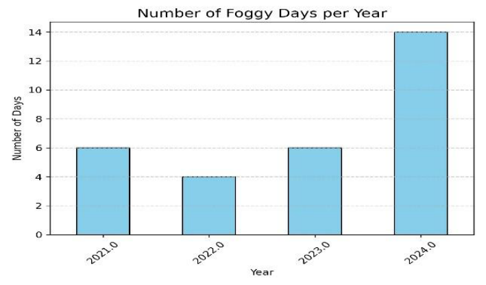 Figure 1A
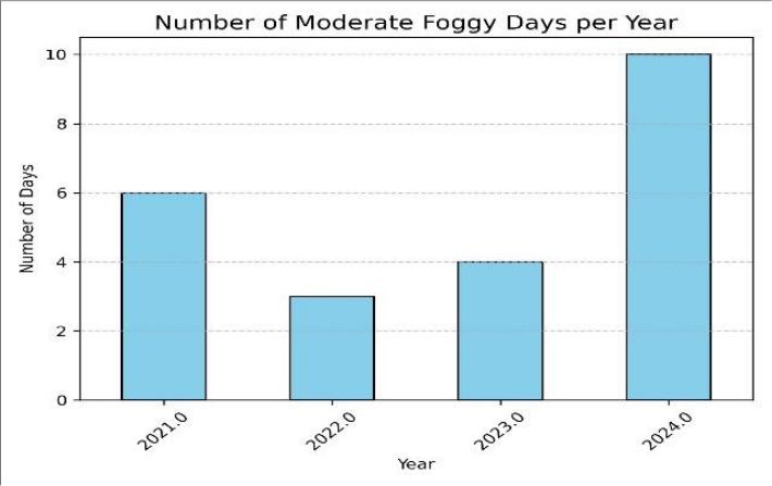 Figure 1B
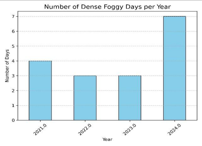 Figure 1C
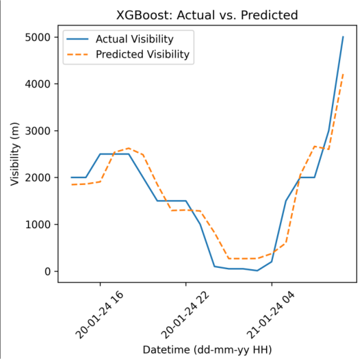 Figure 2A
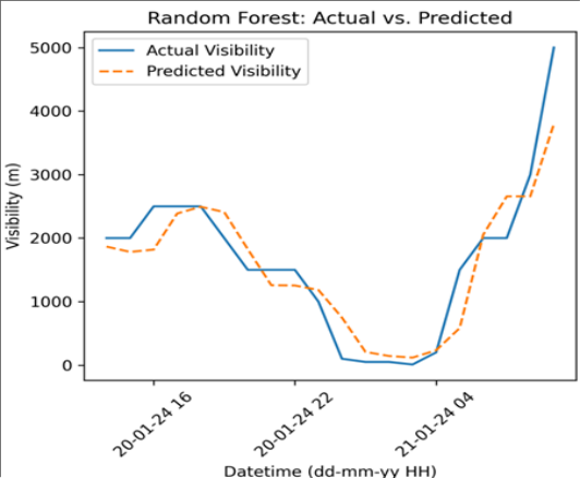 Figure 2B
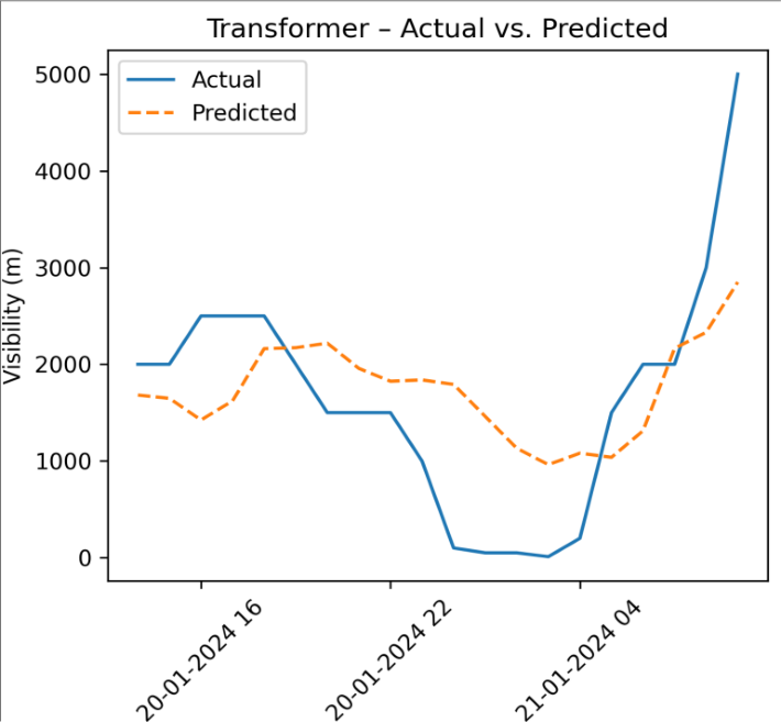 Figure 3
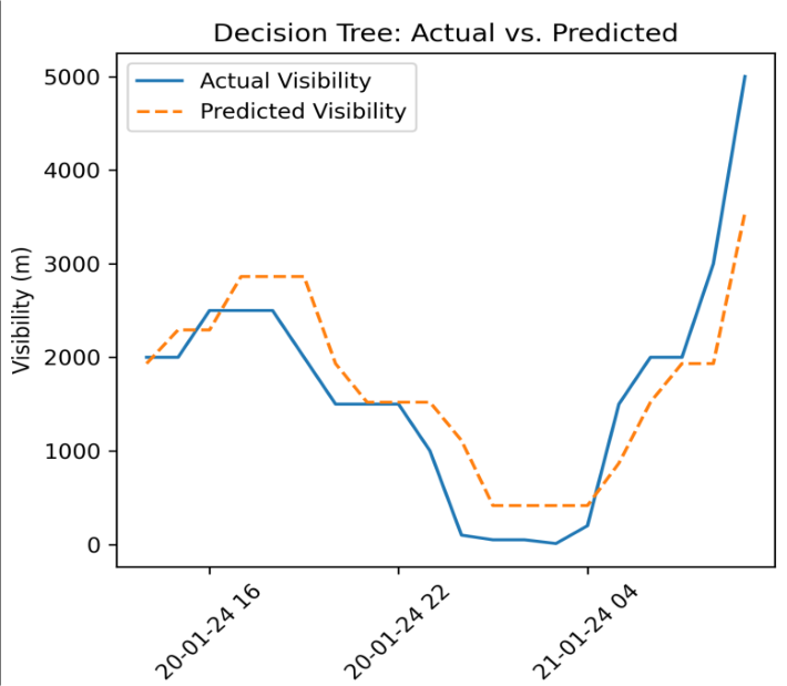 Figure 3
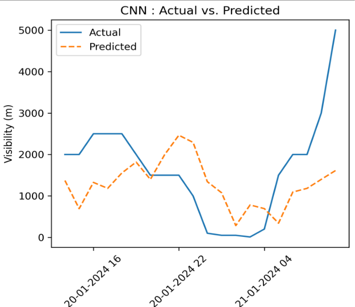 Figure 4
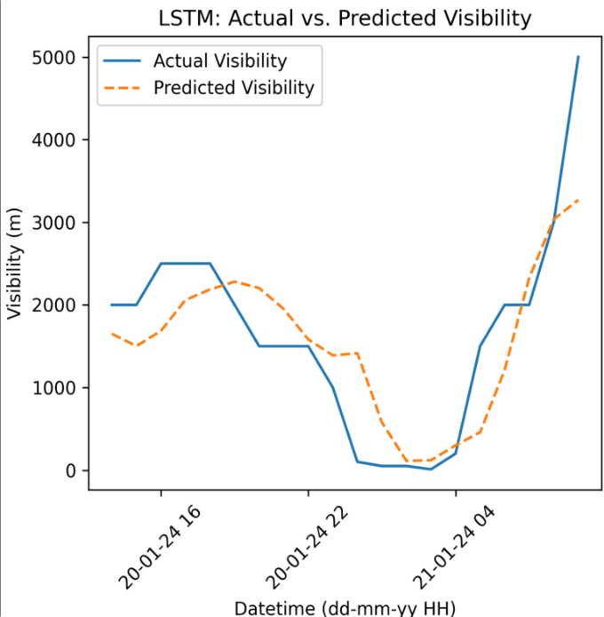 Fig5
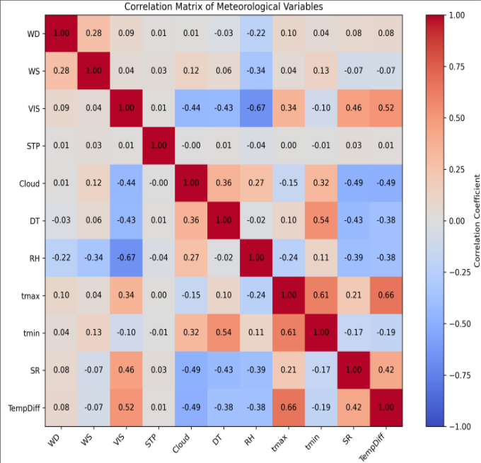 Figure 6
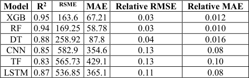 Table 1
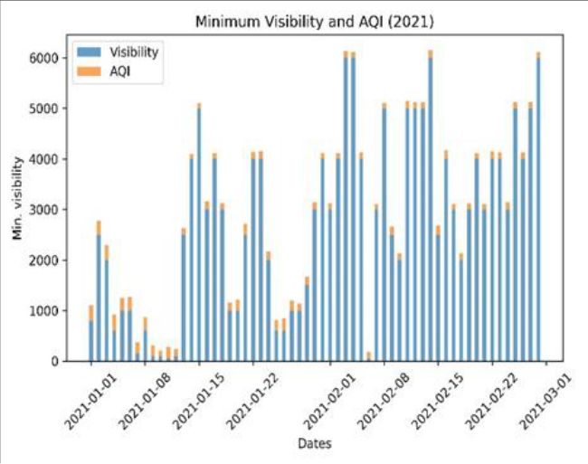 Figure 7
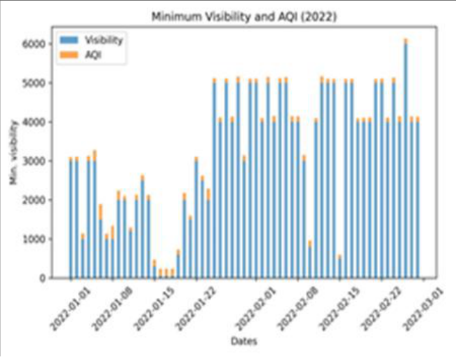 Figure 8
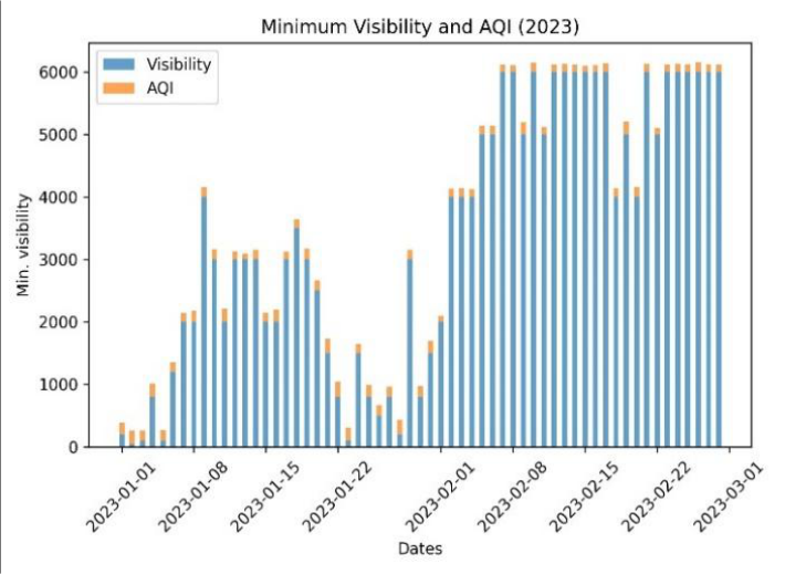 Figure 9
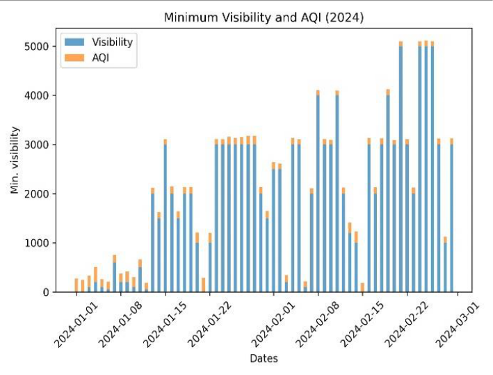 Figure 10
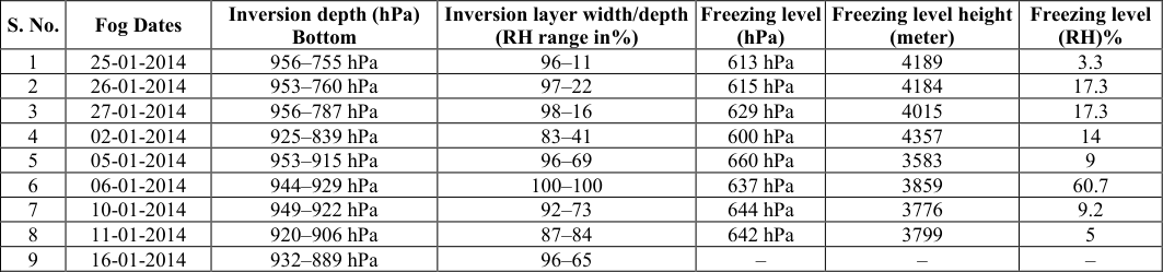 Table 2
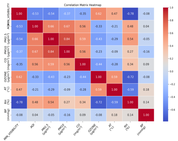 Figure 11
Introduction
Fog is generally a localized phenomenon that matters much as it occurs in morning and daily activities of life, public health, transport including aviation. From recent past decades dense fog events frequency has increased much which have lead to situation of low visibility conditions affected rail, road and air transport difficult and economic activities get negatively affected by it. This for years together raise the concern of the scientific community all over the world has shown keen interest in better understanding of fog (Bendix et al., 1994) [1] . Basically radiation and advection are main types of fog which are most common during winter. The advection fog occurs as wind carries fog from one place to another which is seen in forward sector of western Disturbances (W.Ds), on the other side i.e. rear sector of W.D. the radiation fog occurs that affect North India and some parts of central India during winter [2] . Radiation fog is a result of cooling effect due to long wave terrestrial radiation release by earth and the air close to the ground is warmer compared to adjacent lower layer of air. So in lower few meters air expands following adiabatic process leading to saturation conditions which are conducive for fog. The fog caused by radiation cooling generally disperse a sunrise when the day warms up and inversion breaks as sun's energy get mixed in ambient air. [3] . Clear or less clouded sky and calm or light surface wind and high dew point temperature are factors which support radiation fog and operationally fog is predicted by visibility parameter reported in meters as fog occurs whenever visibility falls below 1000 m along a runway length. Visibility also have diurnal variation and it keeps on changing as the day progresses, radiation fog which is most common over Bhopal disperses in few hours after sun rise.
Local water bodies also have influence on RH availability mainly in surface wind which in turn decides various categories of fog starting from shallow fog and moderate fog further towards severe fog conditions of dense fog and very dense fog. As fog categories depend on horizontal visibility as if it ranges between 1000-500 m shallow fog, 500-201m moderate fog, 200-50 m dense fog and less than 50 m very dense fog [4] . National and international aviation transport services are extremely vulnerable to fog situation. Fog plays important role during landing and takeoff operations and therefore accurate fog predictions are essential for aviation as well as other transport sectors [5] . Fog is crucial for air traffic management and flight planning. Present numerical weather prediction models and other decision support systems, fog prediction is challenging [6] . The fog prediction is difficult due to non availability of data of smaller grid size and the micro-scale factors that produce fog. Atmospheric stability during winter season cause more confinement of particles in lower few meters of height and cooling from below creates low level of inversion which helps in fog formation and its intensification. Increased pollution and fog are posing constant challenges creating critical situation for human health disturbing regular routines of life specially in North and central Indian regions. Few days of persistent cold waves and severe cold waves and intermittent passage of western disturbance fog supports fog in rear sector zone of W.D. as it covers many parts over North India. Winter season low temperature raise energy consumption and increase of burning of organic and inorganic materials raising particulate matter and polluting gases in the atmosphere. Alarming fog situation needs accurate prediction which can be done by doing accurate representation of emissions in atmospheric models for improving the forecast of air quality index (AQI) and fog occurrence. Now a days fog in its extreme conditions disrupt traffic on road and also creates situation of long hours of traffic congestion on highways due to low visibility. Being very dense fog may lead to road accidents and may claim lives. Therefore accurate fog predictions are very essential for addressing ongoing climate extremes [7] . This study spans the winter season meteorological variations along with does the testing of capabilities of recently available tools of machine learning (ML) that can give prediction of Visibility <1000 m as fog event at Raja Bhoj Airport (ICAO Index-VABP), a representative station of Central India [8] . AI based model like XGBoost and Random Forest models which are regression models and also given trial for LSTM (long short term memory), Convolutional Neural Network (CNN) and Decision Tress (DT) which are working on deep learning and checked the training and testing on hourly METAR data. Various research studies have highlighted the transformative potential of AI technologies for fog prediction, with the utilization of current weather data for high accuracy for visibility changes and efficiency compared to traditional NWP models [9] .
Study Area and Data Collection
Bhopal airport is centrally located in India and surrounded with water bodies like small and big lakes, undulating hills, enriching its natural beauty. The Idgah and Shyamala hills are covering northern region, and Katara hills is covering southern region. The two main lakes i.e. Upper lake and lower lake act as main source of moisture and during winter morning time dense fog is seen in parts of city closer to these lakes. As water body remain warmer than adjacent land mass in winter and air in contact with land is at lower temperature than the air in contact with water body. Cool air coming from surround land areas mixing with moisture available over upper and lower lakes creates a situation of vapor coming in contact with cold air initiating rapid condensation and forming tiny water droplets with remain suspended in air in lower atmosphere forming a layer of fog /low cloud near upper lake close to airport area lowering the visibility in morning hours making landing operations difficult at airport. Data is collected from AMO Bhopal and hourly METAR data obtained from CLIMS portal and is used for the study for a period of 2021-2024. The main data parameters are Temperature, Dew Point, Humidity, Pressure (station level, mean sea level), Wind Speed and Direction, Cloud Cover. After concatenating the four datasets, preprocessing steps included dropping columns with excessive missing data and those not relevant to the prediction task. Missing values were imputed using the mean (pre value + post value/2). Upper air data of radiosonde of 00Z and AQI along with pollutants concentration data from CAAQMS located at Paryavaran Parisar, Bhopal through CPCB Ambient Air Quality Real time data Server. The data may also be obtained from using url: https://airquality.cpcb.gov.in/ccr/#/caaqm-dashboard/caaqm-landing. XGBoost being a recent tool of machine learning, which has high efficiency, scalability and also the flexibility [10] . It is able to handle large, structured datasets of various kind and it can provide insights through feature identification and analysis and can handle imbalance of data sets. As compared to other available gradient boosting libraries mainly like LightGBM and CatBoost, XGBoost is better for its balance of speed and accuracy of results, but it also requires more rigorous tuning for optimal performance. Random Forest, which is another ensemble method, is quite simple but generally less powerful compared to XGBoost for complex datasets. Often time series data fails to capture the temporal dependencies in the inherent weather data and to address this issue concept of feature engineering is applied to enhance the quality of the predictions that are projected on test data set and compared with observation of that time period. Only just raw visibility is not enough to predict the next time step visibility. We used the lag features of past 2 hours as the visibility factor does changes gradually. This helps the model to capture the short term variations and persistence. It also includes the rolling means of last 3 and last 6 hours which helps to smooth the noise and capture the local trends in data. It helps the model to detect the gradual patterns in the data, while not just instant changes in the data. The lag features and moving averages convert time series into a structured numeric pattern that helps the ML and DL models to handle the data. Mostly recent neural networks such as RNN and CNN used to process the data in sequential manner while transformers capture long-term dependencies inherited in data set, identify how older values are influencing the newer values in time series and then looks at each time step which affects the visibility at the given time. It is faster than CNN or RNN as it is free from sequential processing and addition of temporal patterns is done to understand the encodings. Each observation looks at each of past observations and weights each of them for the prediction of next values. After this process, the output goes through a small neural network which helps the model to be non-linear. This helps the model to learn the complex relationships from the features. Then the model adds input to back to each layer make training stable. Layer normalization keeps the output scaled neatly. These are all used to improve the ability of model to capture deep patterns. The CNN works on deep learning with convolutional layers, while Transformers include deep learning with self-attention layers. Both models take the time series as the input where CNN captures local variation patterns via convolutions while transformers capture long-term dependencies via selfattention. CNN needs moderate feature engineering as convolution automatically extracts local patterns from data. Transformers with minimal feature engineering as the model learns relationships across different time steps automatically. CNN provide moderate interpretability as compared to Transformers. Transformers take more time to train and tune as compared to CNN as it depends on sequence lengths and layers. Transformers also require large datasets to train for a better generalization. CNN is well suited to predict the temporal features and train the model on multivariate time series data while transformers are more suitable in cases where long-term forecast is to be prepared with multivariate sequences and time series to make the model learn on complex relationships. Predicted visibility with CNN is nearly following the observed visibility trends Fig. 4 during 0000 UTC to 0600UTC and thereafter improvement of visibility is well captured. The low values of visibility below 1000m are missed by model as seen by predicted visibility curve. The decision tree is the model which creates a tree structure to predict next time step values. It needs tabular features as input some with the feature engineering, comprising of adding lags and moving averages by modifying codes as to deal with nonlinear variation of meteorological variables. It is highly efficient on small datasets but not much scalable on large datasets. As it takes less data and time to train itself to understand the variation hidden in data and prone to over fitting. Similar kind of variations seen fig: 3 bottom, as predicted visibility is over shooting observed visibility when visibility is above 2500m during day time 0600UTC and predicted visibility also undershooting during morning time 00UTC when visibility is reducing in actual observation and going below 1000 m. Predicted visibility curve is only showing 1000 m visibility and below that model is not picking the variation which are crucial as fog begins when visibility falls below 1000 m. As Decision tree model is very sensitive to data. It is not suitable for visibility prediction datasets where interpretability is important. Long short term Memory (LSTM) model, is one of the types of recurrent neural networks (RNN) is a deep learning model which has capability to capture the temporal dependency of time series and can be utilized for meteorological fog predictions [10] . Deep LSTM (3 stacked layers), LSTM (128) → LSTM(64) → LSTM(32), with batch normalization for stability and Adam Optimizer (LR = 0.001) for optimization of output variable i.e. visibility [16] .
Methodology
Model has been trained and tested and error estimation of the target output variable from the observed values has been done. Using hourly meteorological data set predicted visibility follows trend of observed visibility follows when observed visibility is in moderate range 1500-4000 m and during low visibility timings i.e, during morning hours predicted visibility follow the reducing trend does not go as low as that of actual observed visibility. As data period is short and fog events with visibility below 500m are limited in number, prediction of low visibility scenario is compromised by LSTM model as evident from Fig. 5. A mixture of smoke with dust, and other pollutants combined with suspended tiny water droplets, resulting in poor visibility and compromise with air quality, especially during winter season [10][11] . The temperature inversion, calm winds, and high moisture trap pollutants close to the ground. Smog forms when fog along with air pollutants (PM₂.₅, PM₁₀, smoke, SO₂, NOx, etc.) combine.
It is generally common in post-monsoon and winter seasons.
A lower visibility can be a result of many natural process and also the response of pollutants to the meteorological parameters during winter season. The air quality index (AQI) is a tool which gives idea about four major pollutants and relates it to human health. How low visibility conditions during moderate to dense fog conditions are linking with AQI values, variation of AQI and variation of minimum visibility attained during a foggy day is an important indicator of impact of fog on air quality and also on human health. To understand the variation of visibility of Bhopal during the past few years and to address the key meteorological parameters affecting the visibility along with interplay of anthropogenic and natural pollutants. Diurnal variation of relative humidity (RH) and the total column water vapor (TCWV) plays a role in fog -haze inter conversion mainly in low-visibility events [18,19] . For this study daily values of AQI revealed that air quality status under defined categories ranging from good, moderate, satisfactory and poor, very poor class used to describe fog conditions and air quality situation in city. Visibility variations are quite high in winter season. Visibility values are high in late January and during middle of February month i.e. 4000 m to 6000 m. and visibility reduces to 50-200 m for few days in January month during dense fog episodes. AQI has less fluctuations as compared to visibility as it is based on pollutants concentration in atmosphere. When AQI attains higher values generally indicates poor air quality, which may or may not be associated with reduction in horizontal visibility [19] . Air quality index variations with minimum visibility observed at airport has been analysed. Out of four years, very low visibility 0-200 m has been observed in first fortnight of January and more often first week of January is prone for dense to very dense fog(fig. 78910). For the year 2021, during dense fog days i.e low visibility 150-50m AQI remains nearly 200-250 range, Moderate fog, AQI attains 300 value and shallow fog conditions AQI reaches nearly 350. During Year 2021 (Fig. 7) AQI increases with visibility increase with fluctuation in foggy conditions while just opposite pattern is seen in 2024, for visibility nearly zero dense fog conditions AQI observed is 300 and for moderate fog days observed AQI is 150-200. While for 2022 (Fig. 8) AQI variations, visibility drops drastically from 300 to50 m but AQI remains high around 170-190. Poor visibility due to high particulate pollution. Visibility improved from 50m to 600m and AQI lowered to value 130, improvement of air quality might be due to winds and better mixing. More cleaned atmospheric conditions the pollutants tend to disperse and generally high visibility links to lower AQI. For 2023 year (Fig. 9), AQI values are almost stable staying mostly between 160-230 while visibility shows extreme fluctuations from very low (~50-100 m) to the maximum (~800 m) many times in season. The minimum visibility is having a negative correlation with RH (-0.78), depicting that higher humidity considerably reduce visibility (fog/haze conditions).Visibility is also impaired by pollutants which are used to define AQI (-0.53), PM2.5 (-0.54), PM10 (-0.37), and CO (-0.35), confirming that increased pollution degrades visibility. A strong positive correlation of visibility with ozone (0.62) and moderate positive correlation with air temperature (0.47) suggest clearer conditions during warmer, photo chemically active periods. BP (pressure) has almost no relationship with visibility (-0.08). AQI is strongly positively correlated with PM2.5 (0.66) and PM10 (0.67), indicating that particulate matter is the dominant driver of AQI and also correlates moderately with CO (0.56). AQI has a moderate positive correlation with RH (0.48), implying worse air quality during humid conditions. A negative correlation with ozone (-0.33) suggests that high-ozone periods do not necessarily coincide with high AQI dominated by particulates. PM2.5 and PM10 are very strongly correlated (0.84), reflecting common sources and atmospheric processes. Carbon mono oxide CO shows moderate correlations with PM2.5 (0.59) and PM10 (0.56) particles, consistent with combustion and other agro residue burnings related emissions. Ozone is negatively correlated with PM2.5 (-0.43) and CO (-0.44), indicating different formation mechanisms (secondary photochemical vs primary emissions). Ozone and temperature are strongly positively correlated (0.59), highlighting temperature-driven photochemical ozone formation. RH is strongly negatively correlated with ozone (-0.72) and temperature (-0.59), typical of cloudy, moist conditions suppressing ozone. Pressure shows weak correlations with most variables, suggesting a limited direct role. Overall conclusion Poor visibility and high AQI are mainly associated with high particulate matter and high humidity. Ozone behaves differently, peaking under warm, dry conditions with better visibility. Meteorology, especially RH and temperature, plays a critical role in modulating both air quality and visibility.
Conclusion
This study comprehensively tested the prominent features of machine learning and deep learning models to predict wintertime low visibility conditions as pre signal of fog over AMO Bhopal and also examined the associated meteorological and air quality data to understand mutual dependencies or influences. The results clearly indicates that models with tree-based schemes of machine learning particularly like XGBoost and Random Forest, perform better as they require less amount of data for their training and produce better results on testing data sets and accuracy with R² values exceeding 0.94 and the lowest error metrics.
Their superior performance highlights their effectiveness in handling limited datasets and capturing the nature of relationships between visibility and meteorological parameters while deep learning based models, like CNN, LSTM, and Transformer are having low prediction skill/ scores as shown in testing of data set because these require large data sets along with better tuning using optimization techniques for prediction of winter fog i.e. low visibility. Moreover low visibility cases are limited so training of these models is on very small data sets which made feature capturing difficult. The meteorological analysis further confirms that wintertime fog i.e. visibility reduction is linked with winter time temperature stratification of upper atmosphere, as cool air being more dense coming in contact with ground and other objects remain at higher temperature than the underlying solid surface causing inversion in few meters from ground. Moderate to dense fog inversion height 3900-4600 meters and inversion layer depth is of the order of pressure difference 200 hpa mainly during January month.
As relative humidity being 95-100 percent on ground remained 86-90 percent till the start of inversion layer in upper atmosphere. The water vapor availability, temperature inversions and saturated lower layers up to 850 hpa level are the main meteorological features of foggy days at AMO Bhopal. The AQI and pollutant accumulation, no doubt played a role in visibility reduction with particulate matter playing a dominant role and AQI does not have one to one link with visibility. Even for zero visibility AQI have values as that of 1000 m and above visibility during morning hours highlighting role of RH. PM 2.5 and PM 10 are important for visibility reduction as dense fog cases are realized in synchronicity PM particle accumulation in air as seen from past four years data. As PM₂.₅ is fine and have been main cause of visibility reduction while PM₁₀ being coarse in size contributed in episodic manner for visibility reduction and as PM10 decreases some improvement in visibility becomes noticeable and our results are also confirming the earlier findings of research [20] . Overall, the findings emphasize that integrating optimized machine learning models with key meteorological and air quality parameters provides a robust framework for operational visibility forecasting, offering valuable support for early warning systems, air quality management, and decision-making in fog-prone regions.
Acknowledgement
AcknowledgementThe author would like to acknowledge Head, CPCB for data of pollutants and Head Meteorological Training Institute, IMD for their continuous support and motivation to carry out this work. Also acknowledge valuable contribution of Yashwant Ingle, department of AI& DS, Vishwakarma Institute of Information technology for constant support during manuscript preparation and Atmospheric Test Bed at Selekhera Sehore (IITM) for upper air data of radiosonde.
Figures and tables from the paper
| Model | R2 | RSME | MAE | Relative RMSE | Relative MAE |
|---|---|---|---|---|---|
| XGB | 0.95 | 163.6 | 67.21 | 0.03 | 0.012 |
| RF | 0.94 | 169.25 | 58.78 | 0.03 | 0.010 |
| DT | 0.88 | 258.92 | 87.8 | 0.04 | 0.016 |
| CNN | 0.85 | 582.9 | 354.6 | 0.13 | 0.08 |
| TF | 0.83 | 565.73 | 429.1 | 0.13 | 0.10 |
| LSTM | 0.87 | 536.85 | 365.1 | 0.11 | 0.08 |
Table text extracted from the original PDF; superscript letters are shown inline. The original table image is below.
View original table image
References
20 in the original paper- Bendix J. Fog climatology of the Po Valley. Rivista di meteorologia aeronautica. 1994;54(3-4):25-36.
- Cho YK, Kim MO, Kim BC. Sea fog around the Korean Peninsula. J Appl Meteorol. 2000;39:24732479.
- Sawaisarje GK, Khare P, Shirke CY, Deepakumar S, Narkhede NM. Study of winter fog over Indian subcontinent: Climatological perspectives. Mausam. 2013;64(3):415-424.
- George PA. India Meteorological Department. Scientific Note. 1948;10(123):119-132.
- LaDochy S. The disappearance of dense fog in Los Angeles: Another urban impact? Physical Geography. 2005;26:177-191.
- Ali K, Momin GA, Tiwari S, Safai PD, Chate DM, Rao PSP. Fog and precipitation chemistry at Delhi, North India. Atmos Environ. 2004;38:4215-4222.
- Singh J, Kant S. Radiation fog over North India during winter from 1989-2004. Mausam. 2006;57(2):271-290.
- Chaurasia S, Sathiyamoorthy V, Shukla BP, Simon B, Joshi PC, Pal PK. Nighttime fog detection using MODIS data over northern India. Meteorol Appl. 2011;18(4):483-494.
- Goswami G, Tyagi A. Advance forecasting of onset, duration and hourly fog intensity over Delhi. Research Report No. RRCM 0714. CSIR Centre for Mathematical Modelling and Computer Simulation; 2007.
- Tenpe KD. Fog over Bairagarh. Indian Journal of Meteorology and Geophysics. 1967;18(4):505-510.
- Niu SJ, Zhao CS, Lu LJ, Yang J. Analysis of the microphysical structure of heavy fog using a droplet spectrometer: a case study. Adv Atmos Sci. 2010;27(6):1259-1275.
- Alsadie D. Artificial Intelligence techniques for securing Fog Computing environments: Trends, challenges, and future directions. IEEE Access. 2024;12:151598-151648.
- Atwal S, Singh D, Chhabra A. Exploring the potential of Artificial Intelligence and Machine Learning in Fog Computing, Cloud Computing and Edge Computing: Benefits and Challenges. In: 2025 International Conference on Intelligent Control, Computing and Communications (IC3). Mathura, India; 2025. p. 199207.
- Singh KD, Singh PD. Machine Learning in Robotics with Fog/Cloud Computing and IoT. EAI/EU: European Alliance for Innovation; 2023.
- Smith J, et al. Advanced Machine Learning techniques for weather prediction. Journal of Atmospheric Sciences. 2023;45(3):234-251.
- Johnson A, Brown M. LSTM networks for time series forecasting in meteorology. Weather Prediction Review. 2022;12(4):89-105.
- Davis R, et al. Deep Learning applications in weather forecasting: A comprehensive review. Artificial Intelligence in Earth Sciences. 2023;8(2):156-178.
- Rajouriya K, Pipal AS, Taneja A. Fog Dynamics in affecting climate and air quality. In: Saxena P, Gupta AK, Sorí R, editors. Fog: Formation, Chemistry, Dynamics, Impact and Dissipation. Singapore: Springer; 2025. p. 115-140.
- Yang Y, Ge B, Chen X, Yang W, Wang Z, Chen H, et al. Impact of water vapor content on visibility: Foghaze conversion and its implications to pollution control. Atmospheric Research. 2021;256:105565.
- Reka S, Singh A, Emmanuel M, Kambala AR, Ramarao MVS, Ram S, et al. Role of meteorology and air pollution on fog conditions over Delhi during the peak winter 2024. The Science of the Total Environment. 2024;954:176478.