
Research article · 2025 · Full text
International Journal of Geography Geology and EnvironmentClassification of the sediments of the Khasa Dam Lake, northeastern Kirkuk, Iraq
Volume 7(10) · Pages 124–134 · DOI: 10.22271/27067483.2025.v7.i10b.437 ↗
Research areasGroundwater and Watershed AnalysisEngineering and Agricultural InnovationsTransboundary Water Resource Management
Abstract
Author-writtenSurface storage dams are their most important source of water. They store water from mountains and valleys on the Earth's surface, constituting a vital resource. Some recent studies have shown that sedimentation can significantly reduce dam efficiency. Unless addressed scientifically, the rapid flow of water from mountainous areas carries with it dirt and small gravel. These materials settle in the lake over time, causing a decrease in the volume of water storage. This problem is observed in many dams in Iraq, especially in the northern regions (Al-Mamooriet al., 2019) [2] and has been studied by Iraqi researchers. This study aims to examine the amount of sediment accumulating in the lake to develop solutions that help preserve water storage for the longest possible period (Hassan, 2018) [1]. Volumetric analysis of sediments within the lake area This study is the first to classify lake sediments The percentages of the volume fractions of clastic sediments (sand, silt, and clay) were extracted using the methods mentioned above. It was noted that silt and clay represented the dominant fractions in the studied samples, while sand represented the secondary fraction, as shown in Table (2). The percentage of clay ranged between (5.1% - 48.4%), with an average of (22.26%), while the percentage of silt ranged between (40% - 62.3%), with an average of (51.96%), and the percentage of sand ranged between (4.7% - 53.4%), with an average of (25.08%). It is clear from the results using mathematical relationships to classify sediments that models We find that most of the samples fall within the quiet water range, indicating that the samples do not move long distances and settle quickly due to the calm water. Samples (9 and 10) also do not follow a specific pattern, indicating that they are deposited by different processes or indicate instability in water movement. Coarse samples (9, 10) have the best sorting and the lowest standard deviation. Fine samples (7, 1, 2) have the worst sorting and the highest standard deviation. This pattern is consistent with sediment transport theories, where long-distance transport processes lead to better sample sorting, and thus the softest and worst-sorted samples.
Summary
Source-checkedPlain-language reading of the full paper, prepared with AI and checked against the text. Each point links to the authors' own words.
Why it matters
- Surface storage dams are critical water resources that collect water from mountains and valleys. View evidence ↗
- Sedimentation from mountainous runoff can reduce dam efficiency by decreasing the available water storage volume. View evidence ↗
- Sedimentation is a recognized problem in many Iraqi dams, particularly those in the northern regions. View evidence ↗
The question
- The study aims to examine sediment accumulation in the Khasa Dam Lake to help develop solutions for preserving water storage. View evidence ↗
What they did
- Ten sediment samples were collected from various locations, including the center and sides of the lake. View evidence ↗
- Wet analysis was performed using at least 250 grams of sample passed through a 0.0625 mm sieve to separate coarse sand from fine clay and silt. View evidence ↗
- The Folk scale was used to calculate statistical coefficients for grain size analysis. View evidence ↗
What they found
- Silt was the dominant fraction (average 51.96%), followed by sand (average 25.08%) and clay (average 22.26%). View evidence ↗
- Based on Folk's classification, most samples were sandy silt or sandy mud, with sample 7 classified as mud. View evidence ↗
- The arithmetic mean of grain sizes ranged from 4.193 Ø to 6.804 Ø (average 5.607), indicating a range from fine sand to very fine silt. View evidence ↗
- All samples exhibited negative symmetry (average -0.298), which indicates a dominance of coarse grains and a medium to high energy environment. View evidence ↗
- Kurtosis values ranged from 0.872 to 1.275 (average 1.08), showing a range from leptokurtic to platykurtic with an overall normal kurtosis. View evidence ↗
What it means
- The authors conclude that most sediments were deposited in quiet water, meaning they settled quickly without traveling long distances. View evidence ↗
- The analysis of the relationship between arithmetic mean and standard deviation indicates that the sediments are of river origin. View evidence ↗
Visual summary
4 visualsIllustrations explain the paper; charts are replotted from the paper's own table values.
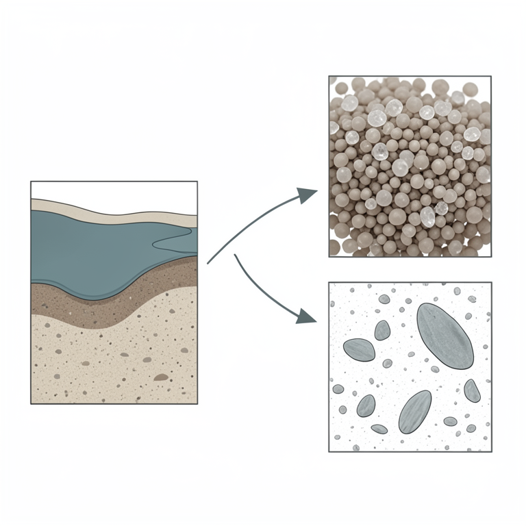
Sediment Composition
AI-generated conceptual illustration (Lake sediment particles (silt, sand, and clay)). It explains the idea and does not show study data.
View source evidence ↗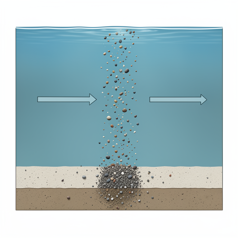
Deposition Process
AI-generated conceptual illustration (lake sediment particles in a freshwater reservoir). It explains the idea and does not show study data.
View source evidence ↗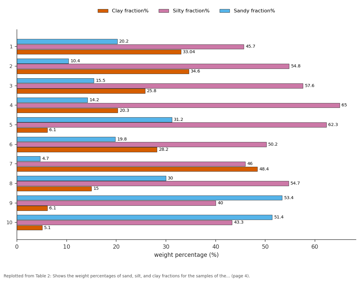
Clay fraction% and Silty fraction% and more: 1 vs 2 vs 3 vs 4 vs 5
Replotted from Table 2 (page 4) of the original paper. Every bar is the paper's own table value.
View source evidence ↗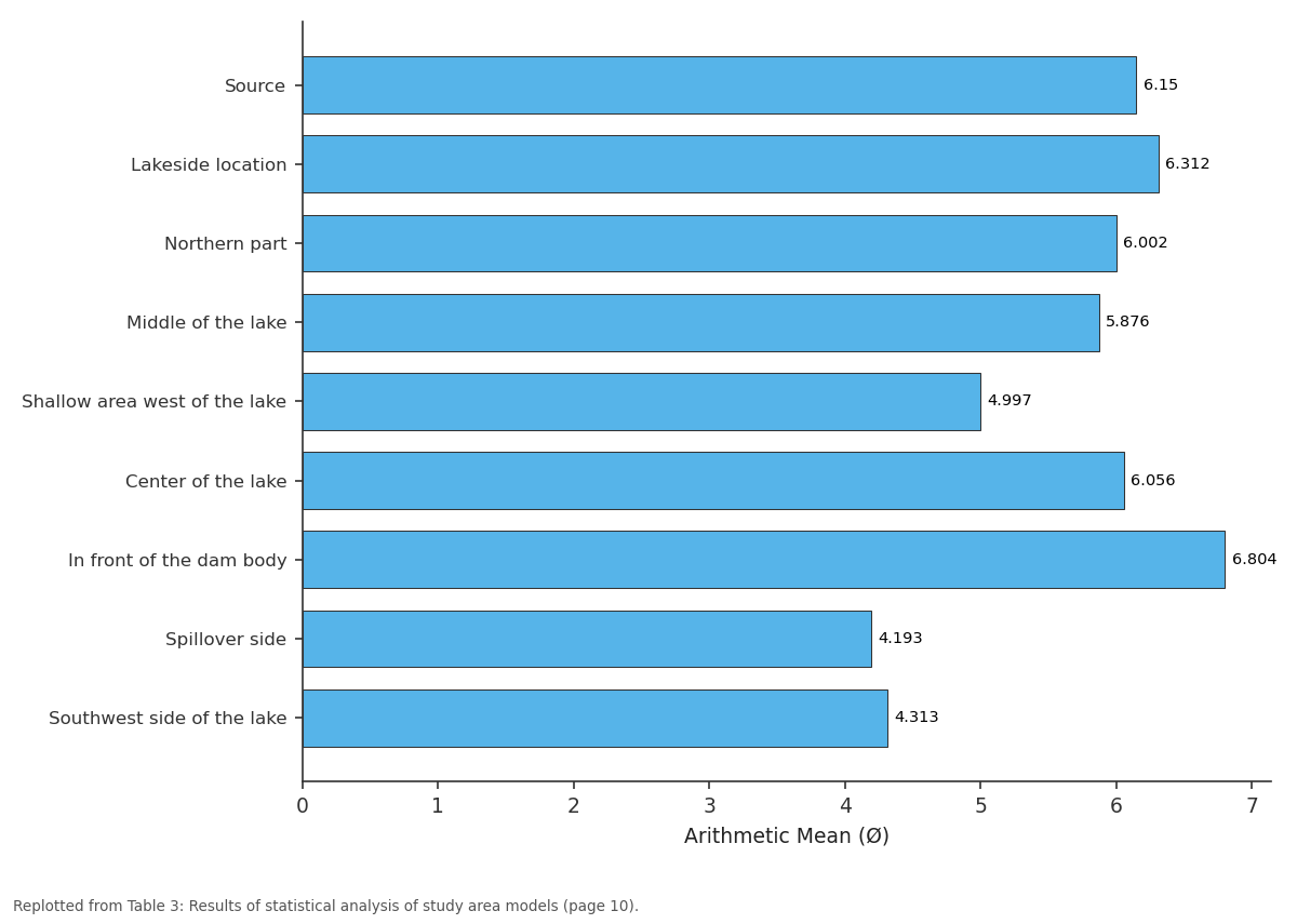
Arithmetic Mean: Source vs Lakeside location vs Northern part vs Middle of the lake vs Shallow area west of...
Replotted from Table 3 (page 10) of the original paper. Every bar is the paper's own table value.
View source evidence ↗Figures & tables
From the original paper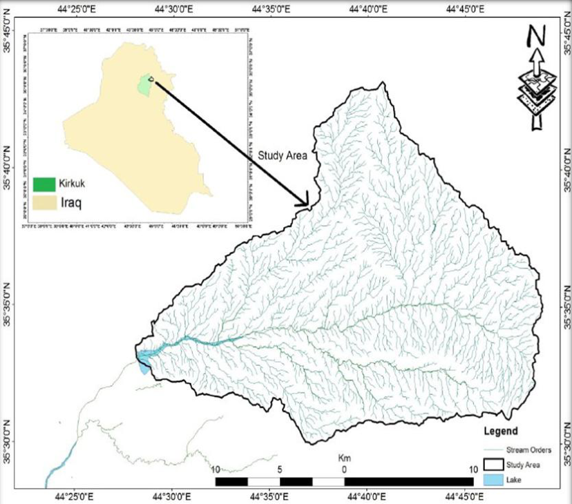 Figure 1
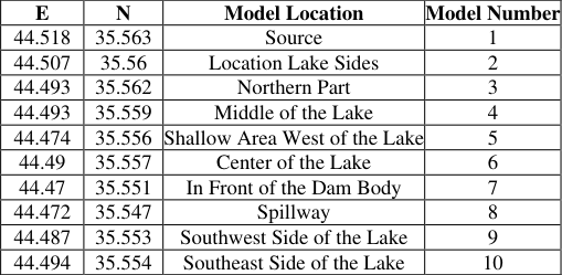 Table 1
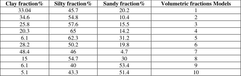 Table 2
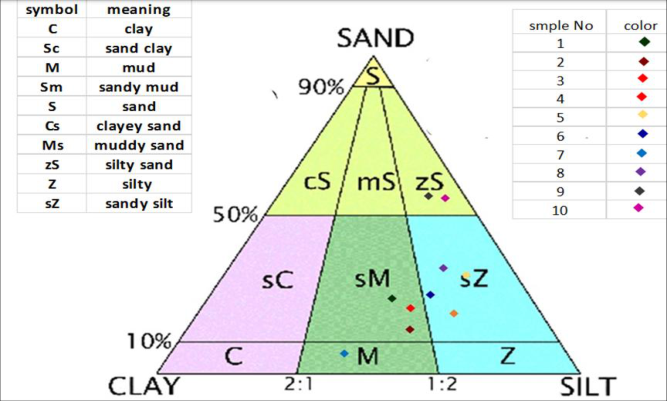 Figure 3
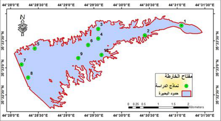 Figure 2
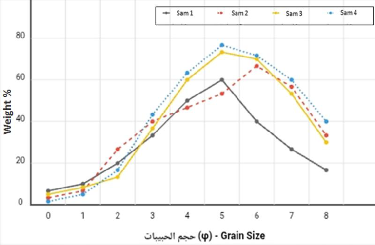 Figure 5
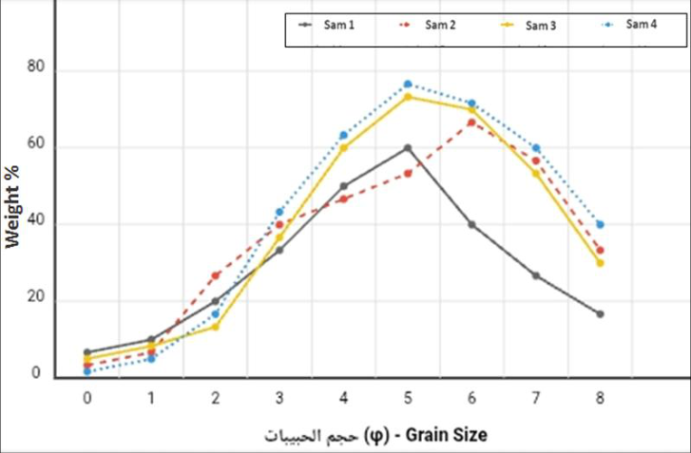 Figure 4
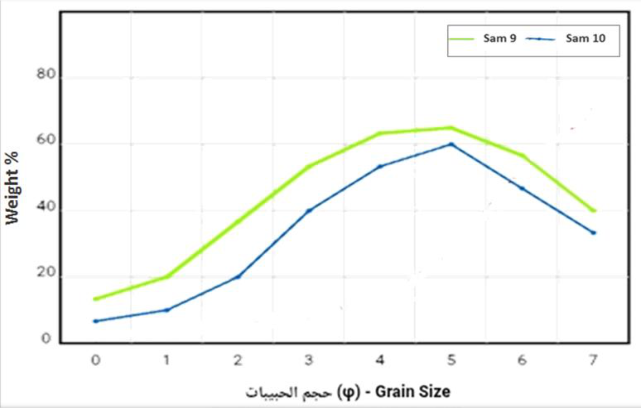 Figure 6
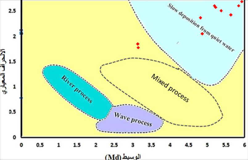 Figure 9
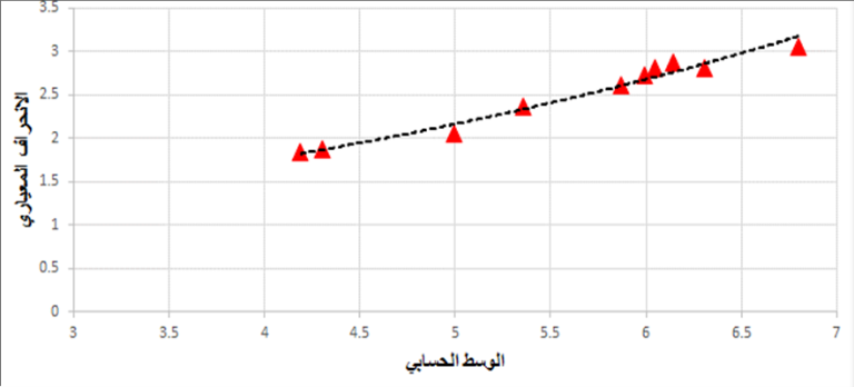 Figure 10
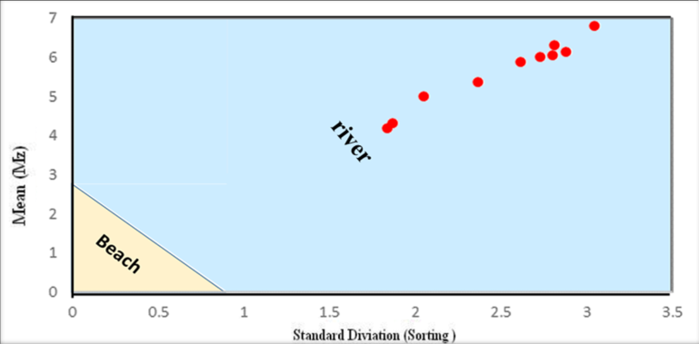 Figure 11
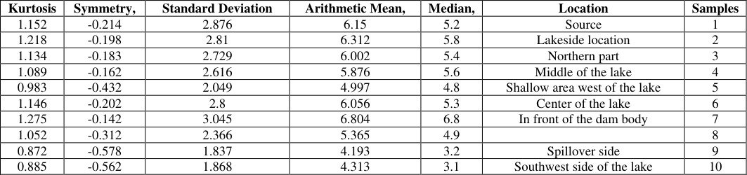 Table 3
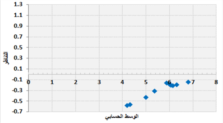 Figure 12
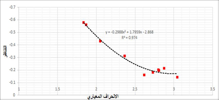 Figure 13
Introduction 1.1 Preface
Surface storage dams are their most important source of water. They store water from mountains and valleys on the Earth's surface, constituting a vital resource. Some recent studies have shown that sedimentation can significantly reduce dam efficiency. Unless addressed scientifically, the rapid flow of water from mountainous areas carries with it dirt and small gravel. These materials settle in the lake over time, causing a decrease in the volume of water storage. This problem is observed in many dams in Iraq, especially in the northern regions (Al-Mamoori et al., 2019) [2] and has been studied by Iraqi researchers. The objective of the research on the private dam lake was to determine the sedimentary characteristics of the reservoir in order to provide recommendations for its optimal use (Hawas, 2012) [3] .
The aim of the study
This study aims to examine the amount of sediment accumulating in the lake to develop solutions that help preserve water storage for the longest possible period (Hassan, 2018) [1] . Volumetric analysis of sediments within the lake area This study is the first to To classify lake sediments
Study Area and Methodology 2.1 Location of the study area
The study area is located northeast of Kirkuk Governorate, with coordinates of latitude (35°33′30″N) and longitude (44°28′30). It occupies an area of approximately 420 km².
The study area is approximately (21) km from the center of Kirkuk city. The study area is bordered to the north and northeast by the northern Jamjamal Fold, to the northwest by the Shwan Sub-Basin, and to the west by the Khasah Dam (Al-Ghuburi, 2020) [4] .
Geology of the study area
Many geological formations are prominent within the study area, covering the region within a different topographic and geomorphological range. All of these formations belong to the Tertiary and Quaternary periods, which extend from the Miocene to the Pleistocene -Holocene. In general, the oldest rocks appear on the edges of the basin in which the study area is located, while modern sediments covered the middle of the basin. 2-3 Stratigraphy of the study area The study area consists of several geological formations and the following is a description of these formations (Sissakian, V.K, 1992) [6] .
Injane Formation (Late Miocene)
The Injana Formation (Upper Fas) is part of the Tertiary geological age, and its stratigraphic location indicates an Upper Miocene age (Al-Naqib, 1959) [8] . It consists of mudstone, siltstone, and sandstone in the study area (Sissakian & Al-Jiburi, 2012) [9] . However, according to (Sissakian et al., 2017) [25] , the thickness of the formation is 398 meters. According to (Kassab and Jassim, 1980) [11] , the Injana Formation contains less information than the Muqaddadiya Formation. The Injana Formation comprises 0.94 square kilometers (0.223%) of the study area.
Muqdadiya Formation (Late Miocene-Pliocene)
The Muqdadiya Formation (Lower Bakhtiari) is considered to have formed during the Tertiary geological period. Using the stratigraphic location, deposits of pebbly sandstone, siltstone, and mudstone were found in the study area (Jassim et al. 1984) [25] (Al-Rawi et al. 1992) [7] . The thickness of the formation is 456 meters (Sissakian et al., 2017) [25] . The Muqdadiya Formation covers an area of 30.59 square kilometers (7.26%) of the study area.
Bai Hassan Formation (Pliocene-Pleistocene)
Using stratigraphic location, the Bai Hassan Formation (Upper Bakhtiari) was identified as belonging to the Pliocene-Pleistocene, a Tertiary geological epoch (Jassim et al. 1984) [26] and (Al-Rawi et al. 1992) [7] . The Bai Hassan Formation consists of sediments that include sandstone and mudstone found in the study area (Jassim et al. 1984) [26] and (Al-Rawi et al. 1992) [7] . The thickness of the formation is (790) mm, and the study area comprises (354.74) square kilometers (84.46%) of the Bai Hassan Formation.
Quaternary (Middle Holocene)
This period is represented by the Quaternary sediments found in the research area. It is characterized by slope deposits containing fine clastic rock fragments, multiple deposits containing silty clay soils, and river terrace deposits with sandstone and mudstone. Quaternary sediments constitute 10% of the research area, equivalent to 12,272 square meters (Sissakian, 1992) [5] .
Tectonic and structural study area
According to the classification made by (Buday and Jassim 1987) [6] , in which the area was separated into a high folded zone and a foothill zone, the research is located within the unstable platform on which tectonics continues in the area. (Bolton, 1958) [12] was the first to propose a foothill zone by virtue of (Doski and Ahmad, 2016).
Geomorphology of the Study Area
Rainfall is the sole source of water in the study area, falling annually during the winter and spring seasons. The area is characterized by a dendritic drainage system, named after the Greek word for "dendritic pattern" (dendron). The drainage pattern often tapers from the highlands toward the main river, or from the north and northeast to the western part of the study area. Weathering and erosion are also widespread in this area, significantly affecting the region. Sheet erosion affects almost all flat areas covered with various sediments. The degree of weathering varies depending on the rock types, and due to the diverse rock types present within the area, all degrees of weathering are present (Sissakian, 1992) [5] .
Topography of the Study Area
The study area contains several small valleys that flow into the main stream. Part of the surface water flows from the higher elevations in the north to the western part of the area, while the other part flows from the northeast of the study area to the western part, where the two sections of the valley meet at coordinates (3936202 East, 464719 North) near the dam.
Collecting Sediment Samples
Traditional methods were used to collect sediment samples from the sides of the lake and dam. Nylon bags were used, and each sample was numbered and recorded, along with the date and time of collection. Sediment samples were collected in polyethylene bags, with their location, number, and date recorded. For samples taken from the center of the lake, a small boat and a large shovel were used to collect samples from as deep as possible. A coring machine was also used on-site to collect samples from depths inaccessible by conventional methods. A GPS device was used to determine sample collection locations. The samples were plotted on a map of the study area using ARCGIS 10.8.
Sediment Analysis
The laboratory work on the sediment section included a volumetric analysis to separate the different sizes of sediments for later use in petrographic studies. The following is a brief description of the processes and analyses conducted in the lab.
Size Analysis
The percentage of different sizes in dry sediment samples can be obtained by grain size analysis (mechanical analysis). This means analyzing the sediment into different size groups. This analysis can be performed in one or two stages. The total number of samples analyzed by size was 10, consisting of samples taken from the sides of the lake and samples taken from the center of the lake. The method (Folk, 1974; Carver, 1971) [13] was used. In the wet analysis, at least 250 grams of the sample was isolated. After dissolving it in distilled water, at least 250 grams of sediment samples were passed through a 0.0625 mm (200.No) sieve. After this procedure, coarse sand particles are separated from fine clay and silt particles. All components must be dried. Therefore, the sediment was analyzed into particles smaller than 0.0625 mm by the wet analysis method. This method is primarily based on the principle of sedimentation using Stoke's Law (Folk, 1974) [13] .
Sieve Analysis
Sieve analysis was conducted for 10 samples distributed over all parts of the lake. Statistical coefficients for grain size were calculated using the Folk scale (Folk & Ward, 1957) [14] . Sieve analysis of sediments is used to calculate percentage values using sieve No. ( 4) or (200 µ). As for smaller sediments, a hydrometer was used to calculate the percentage of clay in the samples. The program (version) was relied upon to provide statistical coefficient values to describe the grain distribution of sediments and the possibility of providing extrapolation of the trend and direction of the distribution of fine-grained sediments (Poppe et al., 2004) [15] . The program inputs are the weight percentages of sand, silt, and clay, using the Phi function (Ø notation), separated from each other by commas. Some analyses were conducted at the College of Science at the University of Kirkuk, and some others were analyzed at the Kirkuk Construction Laboratory. The purpose of analyzing the grain size, whether wet or dry, is to draw the curve. The cumulative use is to determine the percentages of sediments, and the second use is to apply mathematical equations to sediment transport processes. Table (1) and Figure (2) show the location of sampling from the study area.
Results and Discussion
Results and Discussion
Classification of Clastic Sediments
The percentages of the volume fractions of clastic sediments (sand, silt, and clay) were extracted using the methods mentioned above. It was noted that silt and clay represented the dominant fractions in the studied samples, while sand represented the secondary fraction, as shown in Table (2). The percentage of clay ranged between (5.1% -48.4%), with an average of (22.26%), while the percentage of silt ranged between (40% -62.3%), with an average of (51.96%), and the percentage of sand ranged between (4.7% -53.4%), with an average of (25.08%). The percentages were projected onto the classification triangle proposed by (Folk, 1954: In Carver, 1971), Figure (3), in order to know the textural characteristics of the sediments that were withdrawn from the lake. We find from the triangle that most of the samples are located in the sandy
Size-frequency curve
The size-frequency curve is plotted to provide an idea of the grain size distribution (Figure 4), Figure 5, and Figure 6). It can be plotted in various forms, such as unimodal, bimodal, or polydistributive. It may also provide a spectrum of dispersed sizes (Hartmann, 2004) [16] . The curve also provides an idea of sorting and symmetry (Friedman and Johnson, 1982) [17] . When examining the ten samples studied, we observe a diverse spectrum of distributional patterns that reflect the complexity of sedimentary processes. Samples (2, 3, 4, 7, 8, 9, and 10) exhibit a unimodal distribution, indicating the presence of a single dominant transport and deposition mechanism under relatively stable hydrodynamic conditions. This pattern typically reflects a homogeneous sedimentary environment where a single force, such as a water current, sorts grains according to size and density. In contrast, samples 1, 5, and 6 exhibit a bimodal distribution, a more complex pattern that reveals the overlap of multiple sedimentary processes. This pattern may be attributed to the mixing of sediments from two different geological sources, to cyclic changes in water current intensity, or even to the redeposition of older sediments.
Cumulative Frequency Curve
The cumulative frequency curve is an important statistical and sedimentological tool in studying the size distribution of sedimentary grains. It enables the cumulative percentage of grains passing through screens of different sizes to be displayed in the form of a graphic curve. The horizontal axis represents the Phi scale values, which express the grain sizes (Krumbein, 1934) [18] , while the vertical axis represents the cumulative percentage of the total sample weight (Folk & Ward, 1957) [14] . The shapes of the curves reflect the mechanical methods of sediment transport, and thus an idea of the energy of the medium through which sediment is transported. The cumulative curve also includes three clusters, and thus the curve consists of three main lines representing the three mechanics (jumping, stuck, and rolling) (Visher, 1969) [19] . Segmented curves indicate that the sediment contains more than one component. It is noted that most of the curves consist of two main lines, one of which is short and has a slight slope, which represents transport by attachment, and this process is common in the transport of clay and silt grains, and the other line has a high and long slope, indicating transport by jumping, and includes sand grains (Mahdi, 2006) [20] . We notice from Figures (7) [17] . Fig ( 7): Shows the cumulative frequency curve for study models (1, 2, 3, 4, 5) (Friedman et al., 1982) [17] .
Fig ( 8): Shows the cumulative frequency curve for the study models (6, 7, 8, 9, 10).
Statistical Coefficients
The study of statistical coefficients (mean, arithmetic mean, standard deviation, symmetry, and kurtosis) is important in studying sedimentary properties, such as the nature of the source rocks and depositional processes. Statistical coefficients (Folk and Ward, 1957) [14] are used, as they provide better results and include both fine and coarse sizes, using the phi notation function, which was obtained from the previous curves.
Median
It is expressed as the diameter of the grains corresponding to the 50th percentile on the frequency-frequency curve. It can be expressed in mm or as the Ø function. Note that this parameter often does not reflect the total sediment volume, so it is preferable not to rely on it (Folk, 1974) [13] . From the cumulative frequency curves of the studied samples, we find that the median values range between (3.1 -6.8 Ø), with an average of (4.9 Ø). The classification of the samples taken from the lake reservoir ranges from (fine sand to fine silt), with an average of (very fine sand). These values reflect the nature of the sediments in the dam lake. The median values indicate varying sedimentation rates across the lake. Areas with a low median are susceptible to more rapid sedimentation, which may affect the lake's depth and storage capacity over time. This requires periodic monitoring and possibly sediment removal interventions to maintain the dam's efficiency.
The arithmetic mean
It is a mathematical average of the sediment sizes in samples. It is difficult to determine precisely, as it is difficult to calculate the total number of grains in a sample (Boggs, 2006) [21] . However, it is more useful than the median because it covers most grain sizes. The arithmetic mean is calculated using three values for Ø: 16 Ø, which represents one-third of the coarse sizes; 50 Ø, which represents the boundary between the sizes; and 84 Ø, which represents one-third of the fine sizes. The arithmetic mean is expressed by the following equation:
The smaller the grain size, the larger the value of this coefficient. It provides an overview of the energy of the medium, the amount of force applied to the study area, and the role of both wind and water in transporting sedimentary particles. From the model results, we note that the arithmetic mean values range between (4.193 Ø -6.804 Ø), with an average of (5.607). This indicates that the samples range from fine sand to very fine silt, with an average of (Greenstone). This indicates the large distances traveled by sediments in the study area.
Standard deviation
This coefficient expresses the extent of the force that determines and controls the distribution of sediments. Large values indicate poor and limited sediment sorting during the transport and deposition process, while low values of the sorting coefficient indicate good sorting through the energy of the medium, which plays a role in the transport and deposition processes (Boggs, 2006) [21] . The standard deviation is calculated from the relationship:
Standard Diviation = +
Where: Ø 5: is the phi value for the percentage 5%. Ø16: The phi value for the 16% percentile. Ø84: The phi value for the 84% percentile. Ø95: The phi value for the 95% percentile.
The standard deviation values ranged between (1.837 -3.045 Ø) and an average of (2.499). Based on these results, we find that the samples ranged between (poor sorting to very poor) and an average of (very poor sorting). This indicates variable transport energy, multiple sources of sediments, as well as an unstable sedimentation environment.
Symmetry and Diffraction
This coefficient is used to determine the slope of the curve. If the slope is positive, this indicates that the area tends to be a sedimentary area, resulting in an increase in fine sediments and the selective removal of coarser grains. If the slope is negative, this indicates that the area is undergoing erosion and an increase in coarser sediments. A symmetrical curve indicates the presence of both fine and coarse sediments, distributed symmetrically. The symmetry and diffraction coefficients are determined by the following relationship:
Skweness = +
Where: Ø 5: is the phi value for the percentage 5%. Ø16: The phi value for the 16% percentile. Ø50: is the phi value for the percentage 50% Ø84: The phi value for the 84% percentile. Ø95: The phi value for the 95% percentile.
Based on the results obtained for the study samples, we find that symmetry values range between (-0.142, -0.578), with an average of (-0.298), indicating that the samples range between (very fine symmetry and coarse symmetry), with an average of (fine symmetry) (Aljuraisy AM et al, 2024) [24] . We find that all samples have negative symmetry, indicating the dominance of coarse grains. This indicates a medium to high energy sedimentation environment with a predominance of coarse grains.
Kurtosis
This parameter is used to measure the separation ratio between the two ends of the curve. It shows the severity of kurtosis in the volume frequency curve (). It also represents a quantitative measure describing the deviation from the normal distribution. The following relationship expresses this parameter: KG = A curve is considered leptokurtic if the middle part of the curve is better sorted than the tail. If the middle part is less sorted than the tail, the curve is flatter, i.e., platykurtic. If the curve has no kurtosis or curvature along its length, the kurtosis is myzokurtic (Folk, 1974) [13] . From the studied models, the kurtosis values for the studied sample samples ranged between 0.872 and 1.275, with an average of 1.08, i.e., they ranged from leptokurtic to flat or platykurtic, with a normal kurtosis (myzokurtic). This reflects the true differences in grain size distribution among the different samples.
Conclusions 5.1 Relationships between grain size coefficients:
This relationship represents statistical coefficients to determine the quality of the sedimentary environment of the sediments (Friedman, 1962), as well as the processes responsible for sediment transport and deposition.
Relationship between standard deviation (sorting) and median:
This relationship is used to determine the quality of the processes that led to sedimentation. We find that there are three ranges, which indicate the basic processes in sediment deposition: river processes, wave processes, and quiet water processes. This relationship was used to study the relationship between the arithmetic mean and standard deviation of the study models, Figure (9). We find that most of the samples fall within the quiet water range, indicating that the samples do not move long distances and settle quickly due to the calm water. Samples (9 and 10) also do not follow a specific pattern, indicating that they are deposited by different processes or indicate instability in water movement.
Fig 9 : shows the relationship between the standard deviation (sorting) and the median (Stewart, 1958) [22] .
The relationship between the arithmetic mean and the standard deviation
This relationship is important for understanding the relationship between sorting and grain size. The lower the arithmetic mean, the higher the standard deviation (Patro, 1993) [23] , and vice versa, which leads to increased sorting with the increase in the amount of silt and clay in the sediment (Folk & Ward, 1957) [14] . From Figure (10), we find that the relationship is negative: the higher the arithmetic mean (fineness of the grains), the lower the standard deviation (improved sorting). Since the samples in our study area are predominantly sandy, they are very poorly sorted, with the exception of some samples, such as sample No. (7), which is predominantly silt and clay, and which are well sorted. The negative relationship indicates that geological processes that lead to fine grains (erosion, long-distance transport) are associated with improved natural sorting. Coarse samples (9, 10) have the best sorting and the lowest standard deviation. Fine samples (7, 1, 2) have the worst sorting and the highest standard deviation. This pattern is consistent with sediment transport theories, where long-distance transport processes lead to better sample sorting, and thus the softest and worst-sorted samples.
Fig 10:
The relationship between the arithmetic mean and the standard deviation of the sediments of the dam lake reservoir (Folk & Ward, 1957) [14] .
The relationship between the standard deviation and the arithmetic mean is also used to distinguish between sand of coastal or river origin (Friedman, 1967). From Figure (11), we find that the study models are of river origin.
The relationship between the arithmetic mean and symmetry
The relationship between the arithmetic mean and symmetry is studied to determine the correlation between increasing grain size and symmetry. The relationship between them must be directly proportional (Cronan, 1972). Although symmetry is negative and indicates coarse sizes, these values decrease with increasing arithmetic mean. This means the relationship is inverse, indicating irregularity in the sedimentation mechanism (Figure 12).
The relationship between standard deviation and symmetry
The values of standard deviation and symmetry reflect the relationship and correlation of specific grain sizes (coarse, fine, or both). Figure (5-7) shows samples taken from the reservoir of the Special Dam Lake. It is noted that there is an inverse relationship between standard deviation and symmetry, indicating the presence of different grain sizes in the sediments of the study area.
Acknowledgement
AcknowledgmentsPraise be to God, and peace and blessings be upon the most honorable of prophets, his family, and all his companions. This research would not have been completed without the help of God Almighty, to whom I owe the greatest thanks and gratitude. First of all, I would like to express my thanks and gratitude to my esteemed professor, Professor Dr. Soran Nihad Sadiq, for suggesting the research topic and for his wise guidance throughout the research period. I also thank the head, professors, and staff of the Applied Geology Department. I also extend my sincere thanks to the Deanship of the College of Science for the facilities they provided me, which contributed to the completion of the research throughout the study period. Finally, a word of thanks to everyone who contributed to the success of this research. May God reward them on my behalf with all the
Figures and tables from the paper
| E | N | Model Location | Model Number |
|---|---|---|---|
| 44.518 | 35.563 | Source | 1 |
| 44.507 | 35.56 | Location Lake Sides | 2 |
| 44.493 | 35.562 | Northern Part | 3 |
| 44.493 | 35.559 | Middle of the Lake | 4 |
| 44.474 | 35.556 | Shallow Area West of the Lake | 5 |
| 44.49 | 35.557 | Center of the Lake | 6 |
| 44.47 | 35.551 | In Front of the Dam Body | 7 |
| 44.472 | 35.547 | Spillway | 8 |
| 44.487 | 35.553 | Southwest Side of the Lake | 9 |
| 44.494 | 35.554 | Southeast Side of the Lake | 10 |
Table text extracted from the original PDF; superscript letters are shown inline. The original table image is below.
View original table image
| Clay fraction% | Silty fraction% | Sandy fraction% | Volumetric fractions Models |
|---|---|---|---|
| 33.04 | 45.7 | 20.2 | 1 |
| 34.6 | 54.8 | 10.4 | 2 |
| 25.8 | 57.6 | 15.5 | 3 |
| 20.3 | 65 | 14.2 | 4 |
| 6.1 | 62.3 | 31.2 | 5 |
| 28.2 | 50.2 | 19.8 | 6 |
| 48.4 | 46 | 4.7 | 7 |
| 15 | 54.7 | 30 | 8 |
| 6.1 | 40 | 53.4 | 9 |
| 5.1 | 43.3 | 51.4 | 10 |
Table text extracted from the original PDF; superscript letters are shown inline. The original table image is below.
View original table image
| Kurtosis | Symmetry, | Standard Deviation | Arithmetic Mean, | Median, | Location | Samples |
|---|---|---|---|---|---|---|
| 1.152 | -0.214 | 2.876 | 6.15 | 5.2 | Source | 1 |
| 1.218 | -0.198 | 2.81 | 6.312 | 5.8 | Lakeside location | 2 |
| 1.134 | -0.183 | 2.729 | 6.002 | 5.4 | Northern part | 3 |
| 1.089 | -0.162 | 2.616 | 5.876 | 5.6 | Middle of the lake | 4 |
| 0.983 | -0.432 | 2.049 | 4.997 | 4.8 | Shallow area west of the lake | 5 |
| 1.146 | -0.202 | 2.8 | 6.056 | 5.3 | Center of the lake | 6 |
| 1.275 | -0.142 | 3.045 | 6.804 | 6.8 | In front of the dam body | 7 |
| 1.052 | -0.312 | 2.366 | 5.365 | 4.9 | 8 | |
| 0.872 | -0.578 | 1.837 | 4.193 | 3.2 | Spillover side | 9 |
| 0.885 | -0.562 | 1.868 | 4.313 | 3.1 | Southwest side of the lake | 10 |
Table text extracted from the original PDF; superscript letters are shown inline. The original table image is below.
View original table image
References
26 in the original paper- Hassan WF. Hydrological and sediment yield modeling for northern Iraqi watersheds. Arabian Journal for Science and Engineering. 2018;43(12):7589-7600.
- Al-Mamoori SK, Abdulrahman SH, Ali NS. Sedimentation problems in dams in Iraq. Iraqi Journal of Civil Engineering. 2019;13(2):44-55.
- Al-Kawzaji MHH. A hydraulic and sedimentary study of the Dibs Dam reservoir in Kirkuk. 2012.
- Al-Ghuburi MRG. Groundwater vulnerability and risk assessment of upstream Al-Khassa Dam Sub-basin, Kirkuk/NE Iraq [Master's thesis]. Kirkuk: College of Science, University of Kirkuk; 2020.
- Sissakian VK. The geology of Kirkuk Quadrangle Sheet NI-38-2, scale 1:250000. Baghdad: GEOSURV; 1992.
- Buday T, Jassim SZ. The regional geology of Iraq: Tectonism, magmatism and metamorphism. Vol. 2. Baghdad: Geological Survey and Mineral Investigation; 1987. 352 p.
- Al-Rawi YT, Sayyab AS, Al-Jassim JA, Tamar-Agha M, Al-Sammarai AHI, Karim SA, et al. New names for some of the Middle Miocene-Pliocene formations of Iraq (Fatha, Injana, Mukdadiya, and Bai Hassan formations). Iraqi Geological Journal. 1992;25(1):1-7.
- Al-Naqib KM. Geology of southern area of Kirkuk Liwa. Iraq Technical Publication. Iraqi Petroleum Company Ltd.; 1959. 50 p.
- Sissakian VK, Al-Jibouri BS. Stratigraphy of the Low Folded Zone. Iraqi Bulletin of Geology and Mining. 2012;(5):63-132.
- Jassim SZ, Goff JC. Geology of Iraq. Prague: Ministry of the Czech Republic and Heritage Oil Company; 2006. 345 p.
- Kassab IIM, Jassim SZ. The regional geology of Iraq. Baghdad: General Directorate for Geological Survey and Mineral; 1980.
- Bolton C. Geological map. Kurdistan series, Sheet 4, Rania. Site Investigation Company; 1958.
- Folk RL. Petrology of sedimentary rocks. Texas: Hemphill Publishing Company; 1974. 182 p.
- Folk RL, Ward WC. Brazos River bar: a study in the significance of grain size parameters. Journal of Sedimentary Petrology. 1957;27(1):3-26.
- Poppe LJ, Eliason AH, Hastings ME. A Visual Basic program to generate grain-size statistics and to extrapolate particle distributions. Computers & Geosciences. 2004;30(7):791-795.
- Hartmann D. From reality to model: the parameterization problem of particle size distributions. International Workshop, HWK, Delemnhorst; 2004. p. 65-67.
- Friedman GM, Johnson KG. Exercises in sedimentology. New York: John Wiley and Sons; 1982. 208 p.
- Krumbein WC. Size frequency distributions of sediments. Journal of Sedimentary Petrology. 1934;4(2):65-77.
- Visher GS. Grain size distribution and depositional processes. Journal of Sedimentary Petrology. 1969;39(3):1074-1107.
- Mahdi TAR. A sedimentary study of the Injana Formation in the Buqaq, Bashiqa, and Mandan regions of northern Iraq [Master's thesis]. Mosul: University of Mosul; 2006. 129 p.
- Boggs SJ. Principles of sedimentology and stratigraphy. New Jersey: Prentice Hall; 2006. 488 p.
- Stewart HE. Sedimentary reflections of depositional environments in San Miguel Lagoon, Baja California, Mexico. Bulletin of the American Association of Petroleum Geologists. 1958;42(12):2567-2610.
- Patro TN. Combustion study of hydrogen-fueled DI diesel engine: simplified heat release analysis. International Journal of Hydrogen Energy. 1993;18(3):231-241.
- Aljuraisy AM, Abdel Wahab ID. Application of water quality index (WQI) to assess groundwater quality in Kirkuk governorate, Iraq. Int J Adv Chem Res. 2024;6(1):31-37. doi:10.33545/26646781.2024.v6.i1a.165
- Sissakian VK, Al-Jiburi HK, Abdul Jab'bar MF, AlAnsari N. Stratigraphy of Injana Formation (Upper Miocene) in Iraq. Journal of Earth Sciences and Geotechnical Engineering. 2017;7(1):49-78.
- Jassim SZ, Buda AG, Kassab IM. The geology of the Kirkuk Quadrangle, Sheet NI-38-6. Baghdad: Geological Survey of Iraq; 1984.