
Research article · 2025 · Full text
International Journal of Agriculture and Food SciencePrice dynamics of pigeonpea in India: An econometric analysis
Volume 7(9) · Pages 551–557 · DOI: 10.33545/2664844x.2025.v7.i9g.793 ↗
Research areasMigration, Health and TraumaRacial and Ethnic Identity ResearchMigration and Labor Dynamics
Abstract
Author-writtenPigeonpea (Cajanus cajan), a vital pulse crop in India’s agrarian and nutritional landscape, plays a crucial role in food security and rural livelihoods. This study was conducted to analyze the seasonality and market integration of pigeonpea prices in major markets of India, including Kalburgi (Karnataka), Amarawati (Maharashtra), Kanpur (Uttar Pradesh), Junagadh (Gujarat), and Katni (Madhya Pradesh), using monthly data from January 2015 to December 2024. Secondary data on prices and arrivals were sourced from APMCs and the AGMARKNET portal. Seasonal indices were computed using the twelve-month ratio-to-moving-average method to explore price and arrival behavior, while stationarity of the time series was examined using Augmented Dickey-Fuller (ADF) and Phillips-Perron (PP) tests. Market integration was assessed through Johansen’s cointegration test and Granger causality analysis to determine long-run relationships and price leadership among markets. The findings revealed that pigeonpea arrivals peaked between January and March, while price spikes occurred during June to October, confirming an inverse supply-price relationship. All price series were found to be non-stationary at levels but stationary at first differences, indicating I(1) behavior. Johansen’s cointegration results indicated strong long-run market integration, particularly among Kalburgi-Kanpur, Katni-Junagadh, and Amarawati-Kalburgi pairs. Granger causality tests identified both bidirectional and unidirectional price relationships, with Kanpur, Katni, and Kalburgi emerging as influential price-leading markets. Additionally, the study highlighted significant regional variation in arrival trends and volatility: Katni showed strong growth but high volatility, while Kalburgi experienced a sharp decline in arrivals. Kanpur exhibited stable supply patterns with steady growth, making it a key anchor market. The study emphasizes the importance of understanding seasonal trends and market linkages to enhance marketing strategies, support timely policy decisions, and ensure better price realization for pigeonpea farmers. Strengthening inter-market coordination, improving procurement and storage infrastructure, and addressing region-specific challenges will be essential to stabilize prices and promote sustainable growth in the pigeonpea sector.
Summary
Source-checkedPlain-language reading of the full paper, prepared with AI and checked against the text. Each point links to the authors' own words.
Why it matters
- Pigeonpea is a critical pulse crop in India, essential for rural livelihoods and national food security. View evidence ↗
- The crop suffers from persistent price volatility caused by factors like erratic monsoons, pest infestations, and shifting demand. View evidence ↗
The question
- The study aims to analyze the seasonality of pigeonpea prices and the level of market integration across major Indian markets. View evidence ↗
What they did
- The analysis focused on five representative markets: Kalburgi, Katni, Amarawati, Junagadh, and Kanpur. View evidence ↗
- The study used monthly data spanning a ten-year period from January 2015 to December 2024. View evidence ↗
- Seasonal indices for prices and arrivals were calculated using the twelve-month ratio-to-moving-average method. View evidence ↗
- Stationarity of the price series was verified using both Augmented Dickey-Fuller (ADF) and Phillips-Perron (PP) tests. View evidence ↗
- Long-run market relationships and price leadership were assessed using Johansen’s cointegration test and Granger causality analysis. View evidence ↗
What they found
- Pigeonpea arrivals peak between January and March, with February being the most dominant month, while the leanest period occurs from August to November. View evidence ↗
- Prices follow an inverse relationship with supply, peaking from July to November and reaching their lowest points during the peak arrival months of January to March. View evidence ↗
- Price series in all five markets were non-stationary at levels but became stationary after first differencing, indicating I(1) behavior. View evidence ↗
- Strong long-run market integration was found among several pairs, including Kalburgi-Amarawati, Kalburgi-Kanpur, and Kanpur-Katni. View evidence ↗
What it means
- The authors recommend policy interventions in warehousing and infrastructure to stabilize prices and prevent distress sales by farmers. View evidence ↗
Visual summary
3 visualsIllustrations explain the paper; charts are replotted from the paper's own table values.
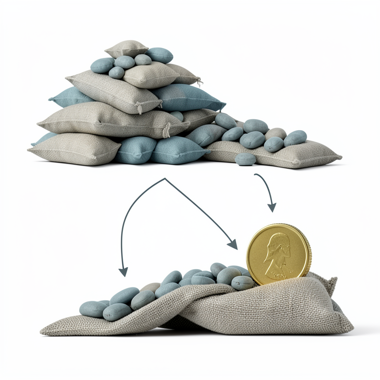
Inverse Supply-Price Relationship
AI-generated conceptual illustration (pigeonpea seeds in burlap sacks). It explains the idea and does not show study data.
View source evidence ↗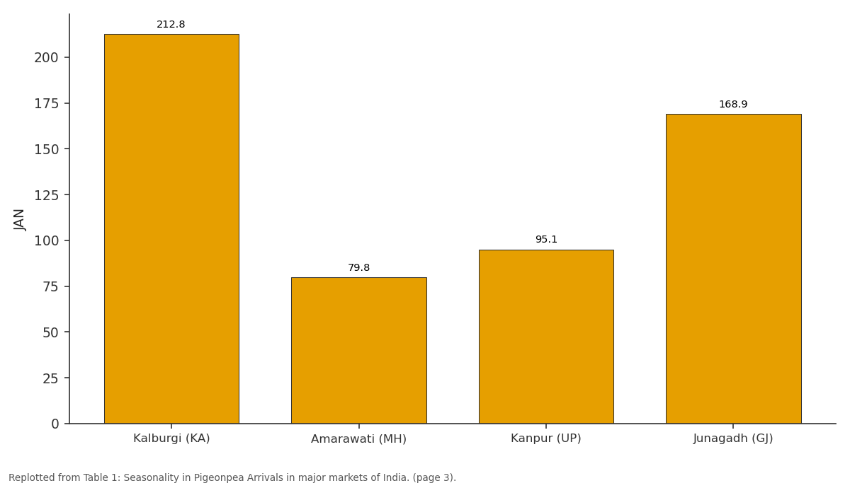
JAN: Kalburgi (KA) vs Amarawati (MH) vs Kanpur (UP) vs Junagadh (GJ)
Replotted from Table 1 (page 3) of the original paper. Every bar is the paper's own table value.
View source evidence ↗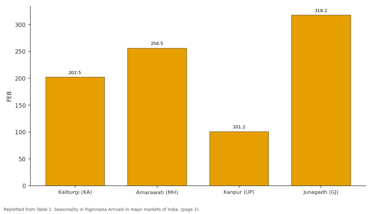
FEB: Kalburgi (KA) vs Amarawati (MH) vs Kanpur (UP) vs Junagadh (GJ)
Replotted from Table 1 (page 3) of the original paper. Every bar is the paper's own table value.
View source evidence ↗Figures & tables
From the original paper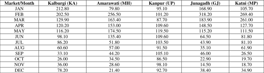 Table 1
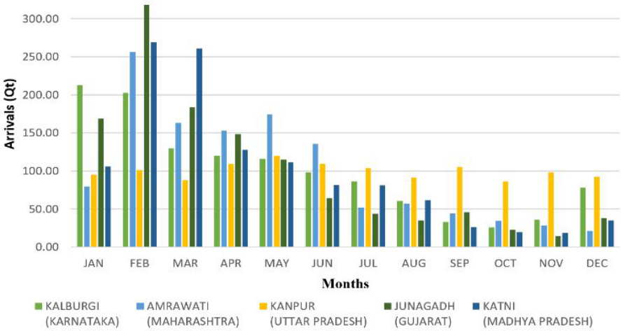 Figure 1
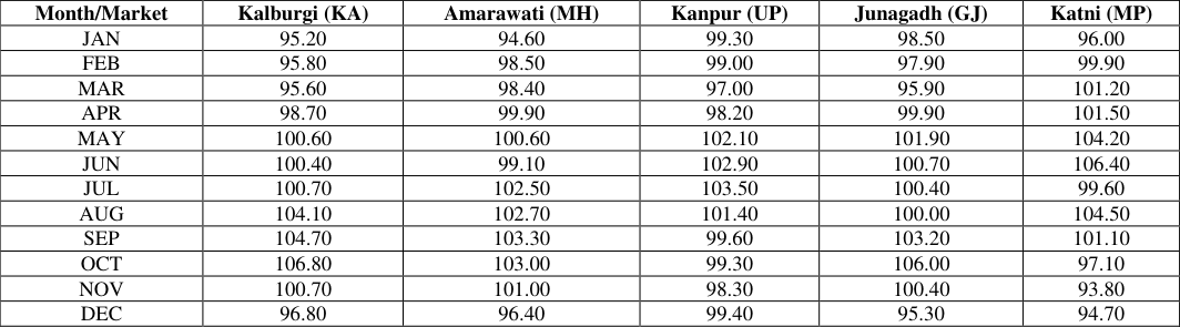 Table 2
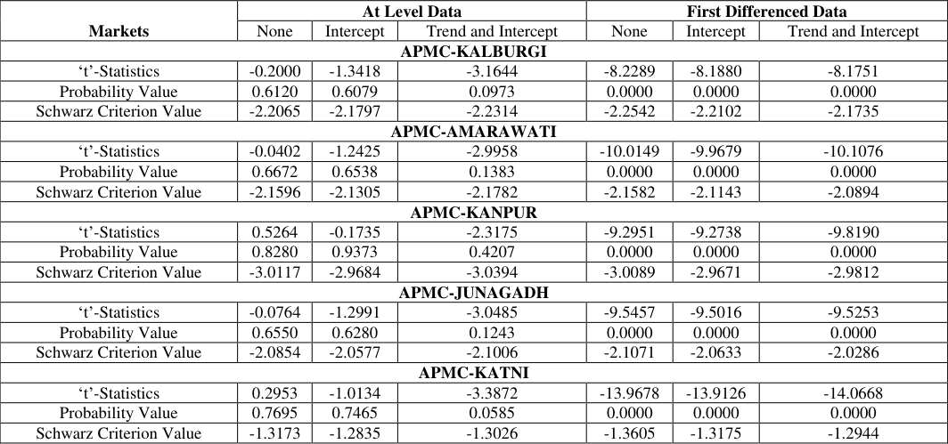 Table 3
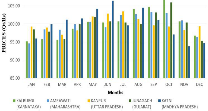 Figure 2
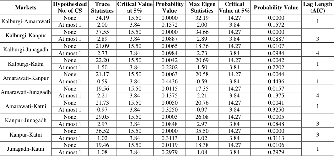 Table 4
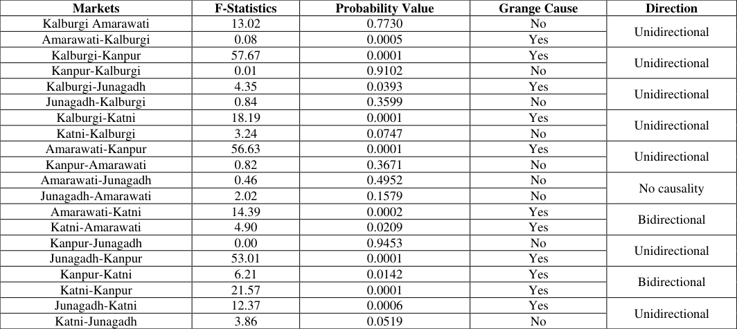 Table 5
Introduction
Pigeonpea (Cajanus cajan L.), commonly known as tur, arhar, or red gram, is a vital pulse crop with significant nutritional, economic, and agronomic importance in India and other tropical and subtropical regions. Recognized for its high protein content, drought tolerance, and nitrogen-fixing ability, pigeonpea plays a key role in ensuring nutritional security, improving soil fertility, and supporting sustainable agricultural systems. India, as both the largest producer and consumer of pigeonpea, contributes approximately 80% of global production, with Karnataka, Maharashtra, Uttar Pradesh, Gujarat, and Jharkhand leading in area and output. In the agricultural year 2023-24, pigeonpea was cultivated over 41.30 lakh hectares in India, yielding 34.16 lakh tonnes, with Karnataka alone accounting for nearly 30% of national production. Despite its multipurpose utility and resilience in marginal farming systems, pigeonpea cultivation and marketing face several challenges. Price volatility is a persistent issue, driven by factors such as erratic monsoons, regional yield disparities, pest infestations, policy interventions, and shifts in domestic and international demand. Although India dominates global production, it still relies on imports to meet growing demand, highlighting the imbalance between production and consumption.
Prices tend to decline during peak arrival months (January-March) and rise during lean periods (June-October), illustrating a clear seasonal price pattern linked to supply fluctuations. Pigeonpea markets across India are increasingly interconnected, with price movements in one region influencing others. This market integration makes it imperative to understand the temporal dynamics, spatial linkages, and volatility patterns of pigeonpea prices. Such insights are crucial not only for farmers aiming to time their sales for maximum returns, but also for policymakers, traders, and market participants seeking to stabilize prices, ensure efficient procurement, and plan buffer stock operations. Analyzing historical trends helps in improving marketing strategies, informing infrastructure investments, and implementing timely government interventions, thereby fostering a more resilient and equitable pulse marketing system. Therefore, the present study has undertaken with following specific objective: 1. To know the seasonality in Pigeonpea prices in major markets of India. 2. To know the market integration among the major Pigeonpea markets of India.
Methodology Data Sources
This study utilizes authoritative secondary data sources to ensure analytical validity. Monthly time-series data on Pigeonpea prices and arrivals were extracted from major Agricultural Produce Market Committees (APMCs) and the AGMARKNET portal. Pigeonpea was selected as the focal crop due to its status as India's largest oilseed in terms of cultivated area, production volume, and contribution to agricultural gross value added. The research is confined to five major producing states Karnataka, Madhya Pradesh, Maharashtra, Gujarat, and Uttar Pradesh, and from each, one representative market was chosen based on the triennium average of arrivals: Kalburgi, Katni, Amarawati, Junagadh, and Kanpur, respectively. The study period spans January 2015 to December 2024.
Analytical Tools Seasonality Analysis
Monthly data on wholesale prices and market arrivals were utilized to analyze the seasonal patterns in the selected markets. To quantify the seasonal fluctuations in both prices and arrivals, seasonal indices were derived using the twelvemonth ratio-to-moving-average technique.
Step I, involved calculating the 12-month moving totals, which were then divided by 12 to obtain the corresponding moving averages. These moving averages were further refined into a series of centred moving averages. A time span of 10 years of data was used for the computation of seasonal indices.
Step II converted the original monthly values into percentages relative to their respective centred moving averages. This step also involved eliminating the irregular components from the time series. The resulting percentages were then grouped by month, and average values for each month were computed.
Step III included adjusting the monthly average indices so that their total equalled 1200. This can be done by working out a correction factor and multiplying the average for each month by this correction factor. The correction factor (K) is worked out as follows,
Where, K is a correction factor S is the sum of average indices for 12 months Multiply K with the percentage of moving average for each month to obtain the seasonal indices.
Market co-integration
Testing of stationarity in price series.
To address the issue of spurious regression that could result from non-stationarity, this study initially tested the stationarity of the time series data using the Augmented Dickey-Fuller (ADF) test. Before investigating any longterm equilibrium relationships among price series through co-integration techniques, it was necessary to confirm that the data were stationary. This step served as the foundation for all subsequent time series analyses. The ADF unit root test, developed by Dickey and Fuller (1979), was employed to identify whether a unit root existed in the data. The presence of a unit root at level form indicated nonstationarity. In such cases, the series was differenced once, and the ADF test was reapplied to assess whether the differenced series had achieved stationarity. The ADF test is estimated using the following regression equation:
Where, P = Prices in each market The null hypothesis in this context stated that the time series contained a unit root, indicating non-stationarity. In contrast, the alternative hypothesis asserted that no unit root was present, implying that the series was stationary. Similar to the ADF test, PP test indicated the presence of a unit root at the level form, it suggested that the time series was non-stationary. In such cases, the series was transformed through first differencing, and the test was reapplied to the differenced series to determine stationarity.
Co-integration analysis using Johanson procedure
The Johansen cointegration test is a widely used statistical method for evaluating the existence and strength of longterm equilibrium relationships among non-stationary time series variables. This approach is applicable only when the time series are integrated of the same order, typically stationary at first difference. The Johansen framework includes two key techniques for determining cointegration: the Trace test and the Maximum Eigen value test. (Johansen, 1988; Johansen and Juselius, 1990) [4,5] The model with n variable vectors was given as,
Where, 𝑥𝑡, ε t are (n×1) vectors, 𝐴𝐼 is (n×n) matrix of parameter, I is (n×n) identity matrix
We test the rank of 𝐴 1 -I matrix i.e., ∏ = A 1 -I. If the rank is Π=k, then the series is stationary in nature. If the rank is 𝛱<𝑘, also known as reduced rank, then there exists cointegration among the series
Granger Causality Test
The presence and causality direction of long-run market price relationship can be assessed by using the Granger causality test directed within vector auto regressive (VAR) model. To perform the Granger causality analysis, an Autoregressive Distributed Lag (ADL) model was specified as follows: These findings are consistent with those of Singh and Sikka (2017) [12] , who also reported high seasonality in pigeonpea arrivals across APMCs in Maharashtra and Madhya Pradesh, with peak inflows occurring from January to March and minimal arrivals during August to November. Similarly, Balai et al. (2021), in their study on lentil arrivals in KUMS Bundi, observed a comparable seasonal trend, with peak arrivals between February and June. Overall, the analysis confirms a distinct seasonal pattern in pigeonpea marketing across India, driven by regional harvesting schedules and supply chain dynamics. These insights are crucial for developing effective procurement strategies, improving warehousing and distribution systems, and enabling farmers to make informed decisions about the timing of market participation to maximize price realization.
Seasonal indices of market prices of Pigeonpea in major markets of India
Seasonal indices of monthly market prices for pigeonpea were estimated using the 12-month moving average method to understand the long-term price behavior and seasonal fluctuations in key producing markets. These indices provide insight into cyclical price movements influenced by supply cycles, consumer demand, and broader market dynamics. The seasonal indices of pigeonpea prices across the selected markets are presented in Table 2. In the Kalburgi (Karnataka) market, the highest price index was recorded in October (106.80), while the lowest was observed in January (95.20), indicating a significant price rise during the lean post-monsoon period. Similarly, in Amarawati (Maharashtra), the maximum price index was also seen in October (103.30), while the lowest was in January (94.60), reflecting a consistent pattern of higher prices during the second half of the year. In the Junagadh (Gujarat) market, prices peaked in November with an index of 106.00, and were lowest in February (97.90), aligning with reduced availability post-harvest. The Kanpur (Uttar Pradesh) market showed a distinct trend, with the highest price index in July (103.50) and the lowest in March (97.00), likely influenced by regional supply timing and demand fluctuations. The Katni (Madhya Pradesh) market registered the highest seasonal index in July (106.40), while the lowest was recorded in November (93.80), suggesting price pressure during post-harvest influx and a spike in midyear due to declining stock levels. All markets exhibited relatively higher pigeonpea prices from July to October, while lower prices were typically observed from November to February, coinciding with peak arrival periods. This seasonal price movement reflects typical market behavior where prices rise during the lean supply period due to reduced availability and increased demand, particularly during the monsoon and festive seasons. Conversely, prices tend to drop during post-harvest months when supply increases. The seasonal indices, illustrated in Figure 2, further reinforce this trend, showing that prices generally rise from May to October, peaking in September to November depending on the market, and decline thereafter. For example, Kalburgi and Amarawati showed peaks in October, Junagadh in November, and Kanpur and Katni peaked during July, before declining in the subsequent months. These findings are supported by earlier studies. Kumawat and Meena (2021) reported that pigeonpea prices in major APMCs of Rajasthan typically peaked between September and November, while the lowest prices were during the post-harvest window of January to March, confirming the seasonal nature of price behavior. Similarly, Purushottam et al. (2013) observed that pigeonpea prices in Kanpur were lowest in July-August and peaked in February and March, emphasizing regional differences in price cycles based on harvest timing and storage practices. Overall, the analysis reveals a clear and consistent seasonal price pattern for pigeonpea across markets. Prices tend to be highest during the monsoon to early post monsoon period (July to November) and lowest during the peak arrival months (January to March). Understanding these patterns is essential for farmers, traders, and policymakers to optimize storage, marketing, and procurement decisions, ultimately enhancing market efficiency and farmer income.
| Month/Market | Kalburgi (KA) | Amarawati (MH) | Kanpur (UP) | Junagadh (GJ) | Katni (MP) |
|---|---|---|---|---|---|
| JAN | 95.20 | 94.60 | 99.30 | 98.50 | 96.00 |
| FEB | 95.80 | 98.50 | 99.00 | 97.90 | 99.90 |
| MAR | 95.60 | 98.40 | 97.00 | 95.90 | 101.20 |
| APR | 98.70 | 99.90 | 98.20 | 99.90 | 101.50 |
| MAY | 100.60 | 100.60 | 102.10 | 101.90 | 104.20 |
| JUN | 100.40 | 99.10 | 102.90 | 100.70 | 106.40 |
| JUL | 100.70 | 102.50 | 103.50 | 100.40 | 99.60 |
| AUG | 104.10 | 102.70 | 101.40 | 100.00 | 104.50 |
| SEP | 104.70 | 103.30 | 99.60 | 103.20 | 101.10 |
| OCT | 106.80 | 103.00 | 99.30 | 106.00 | 97.10 |
| NOV | 100.70 | 101.00 | 98.30 | 100.40 | 93.80 |
| DEC | 96.80 | 96.40 | 99.40 | 95.30 | 94.70 |
Table text extracted from the original PDF; superscript letters are shown inline. The original table image is below.
View original table image
Augumented Dickey-Fuller (ADF) test
The Augmented Dickey-Fuller (ADF) test, a standard method for detecting unit roots, was employed to statistically verify the stationarity of pigeonpea prices in these major markets for Johansen co-integration analysis, and the results are summarized in Table 3. The ADF test showed that the price series for all five major Pigeonpea markets Kalburgi (Karnataka), Amarawati (Maharashtra), Kanpur (Uttar Pradesh), Junagadh (Gujarat), and Katni (Madhya Pradesh) were non-stationary in their level form across all model specifications (None, Intercept, and Trend and Intercept), as the test statistics did not exceed the corresponding critical values. The presence of high pvalues further supported the failure to reject the null hypothesis of a unit root. However, when the series were tested in their first-differenced form, the ADF test statistics for all markets were highly significant under every model specification, with p-values of 0.0000 in each case. The test statistics were more negative than the critical values at both the 5% and 1% significance levels, leading to the rejection of the null hypothesis. This confirms that the Pigeonpea price series became stationary after first differencing in each market.
| Markets | At Level Data | — | — | First Differenced Data | — | — |
|---|---|---|---|---|---|---|
| None | Intercept | Trend and Intercept | None | Intercept | Trend and Intercept | |
| APMC-KALBURGI | ||||||
| ‘t’-Statistics | -0.2000 | -1.3418 | -3.1644 | -8.2289 | -8.1880 | -8.1751 |
| Probability Value | 0.6120 | 0.6079 | 0.0973 | 0.0000 | 0.0000 | 0.0000 |
| Schwarz Criterion Value | -2.2065 | -2.1797 | -2.2314 | -2.2542 | -2.2102 | -2.1735 |
| APMC-AMARAWATI | ||||||
| ‘t’-Statistics | -0.0402 | -1.2425 | -2.9958 | -10.0149 | -9.9679 | -10.1076 |
| Probability Value | 0.6672 | 0.6538 | 0.1383 | 0.0000 | 0.0000 | 0.0000 |
| Schwarz Criterion Value | -2.1596 | -2.1305 | -2.1782 | -2.1582 | -2.1143 | -2.0894 |
| APMC-KANPUR | ||||||
| ‘t’-Statistics | 0.5264 | -0.1735 | -2.3175 | -9.2951 | -9.2738 | -9.8190 |
| Probability Value | 0.8280 | 0.9373 | 0.4207 | 0.0000 | 0.0000 | 0.0000 |
| Schwarz Criterion Value | -3.0117 | -2.9684 | -3.0394 | -3.0089 | -2.9671 | -2.9812 |
| APMC-JUNAGADH | ||||||
| ‘t’-Statistics | -0.0764 | -1.2991 | -3.0485 | -9.5457 | -9.5016 | -9.5253 |
| Probability Value | 0.6550 | 0.6280 | 0.1243 | 0.0000 | 0.0000 | 0.0000 |
| Schwarz Criterion Value | -2.0854 | -2.0577 | -2.1006 | -2.1071 | -2.0633 | -2.0286 |
| APMC-KATNI | ||||||
| ‘t’-Statistics | 0.2953 | -1.0134 | -3.3872 | -13.9678 | -13.9126 | -14.0668 |
| Probability Value | 0.7695 | 0.7465 | 0.0585 | 0.0000 | 0.0000 | 0.0000 |
| Schwarz Criterion Value | -1.3173 | -1.2835 | -1.3026 | -1.3605 | -1.3175 | -1.2944 |
Table text extracted from the original PDF; superscript letters are shown inline. The original table image is below.
View original table image
To ensure the robustness and reliability of the stationarity findings, the Phillips-Perron (PP) test, an alternative unit root testing approach, was also applied alongside the Augmented Dickey
Figures and tables from the paper
| Market/Month | Kalburgi (KA) | Amarawati (MH) | Kanpur (UP) | Junagadh (GJ) | Katni (MP) |
|---|---|---|---|---|---|
| JAN | 212.80 | 79.80 | 95.10 | 168.90 | 105.70 |
| FEB | 202.50 | 256.50 | 101.20 | 318.20 | 269.40 |
| MAR | 129.90 | 163.40 | 87.70 | 183.90 | 261.00 |
| APR | 120.20 | 153.00 | 109.60 | 148.50 | 127.70 |
| MAY | 116.20 | 174.50 | 119.50 | 115.20 | 111.50 |
| JUN | 98.10 | 135.40 | 109.60 | 64.50 | 81.80 |
| JUL | 86.20 | 51.80 | 103.50 | 43.90 | 81.10 |
| AUG | 60.60 | 57.00 | 91.50 | 35.10 | 61.90 |
| SEP | 33.10 | 44.20 | 105.10 | 46.00 | 26.50 |
| OCT | 26.00 | 34.50 | 86.50 | 22.90 | 19.70 |
| NOV | 36.00 | 28.60 | 98.10 | 14.50 | 18.70 |
| DEC | 78.20 | 21.40 | 92.70 | 38.40 | 34.90 |
Table text extracted from the original PDF; superscript letters are shown inline. The original table image is below.
View original table image
| Markets | Hypothesized No. of CS | Trace Statistics | Critical Value at 5% | Probability Value | Max Eigen Statistics | Critical Value at 5% | Probability Value | Lag Length (AIC) |
|---|---|---|---|---|---|---|---|---|
| Kalburgi-Amarawati | None | 34.19 | 15.50 | 0.0000 | 32.19 | 14.27 | 0.0000 | 1 |
| At most 1 | 2.00 | 3.84 | 0.1572 | 2.00 | 3.84 | 0.1572 | ||
| Kalburgi-Kanpur | None | 37.55 | 15.50 | 0.0000 | 34.66 | 14.27 | 0.0000 | 3 |
| At most 1 | 2.89 | 3.84 | 0.0887 | 2.89 | 3.84 | 0.0887 | ||
| Kalburgi-Junagadh | None | 21.09 | 15.50 | 0.0065 | 18.36 | 14.27 | 0.0107 | 4 |
| At most 1 | 2.73 | 3.84 | 0.0984 | 2.73 | 3.84 | 0.0984 | ||
| Kalburgi-Katni | None | 22.20 | 15.50 | 0.0042 | 20.69 | 14.27 | 0.0042 | 1 |
| At most 1 | 1.50 | 3.84 | 0.2202 | 1.50 | 3.84 | 0.2202 | ||
| Amarawati-Kanpur | None | 21.17 | 15.50 | 0.0063 | 20.58 | 14.27 | 0.0044 | 1 |
| At most 1 | 0.59 | 3.84 | 0.4436 | 0.59 | 3.84 | 0.4436 | ||
| Amarawati-Junagadh | None | 19.56 | 15.50 | 0.0115 | 17.35 | 14.27 | 0.0157 | 4 |
| At most 1 | 2.21 | 3.84 | 0.1375 | 2.21 | 3.84 | 0.1375 | ||
| Amarawati-Katni | None | 21.73 | 15.50 | 0.0050 | 20.76 | 14.27 | 0.0041 | 1 |
| At most 1 | 0.97 | 3.84 | 0.3250 | 0.97 | 3.84 | 0.3250 | ||
| Kanpur-Junagadh | None | 29.05 | 15.50 | 0.0003 | 26.08 | 14.27 | 0.0005 | 3 |
| At most 1 | 2.97 | 3.84 | 0.0848 | 2.97 | 3.84 | 0.0848 | ||
| Kanpur-Katni | None | 36.52 | 15.50 | 0.0000 | 35.50 | 14.27 | 0.0000 | 3 |
| At most 1 | 1.02 | 3.84 | 0.3113 | 1.02 | 3.84 | 0.3113 | ||
| Junagadh-Katni | None | 19.46 | 15.50 | 0.0119 | 18.38 | 14.27 | 0.0106 | 1 |
| At most 1 | 1.08 | 3.84 | 0.2979 | 1.08 | 3.84 | 0.2979 |
Table text extracted from the original PDF; superscript letters are shown inline. The original table image is below.
View original table image
| Markets | F-Statistics | Probability Value | Grange Cause | Direction |
|---|---|---|---|---|
| Kalburgi Amarawati | 13.02 | 0.7730 | No | Unidirectional |
| Amarawati-Kalburgi | 0.08 | 0.0005 | Yes | |
| Kalburgi-Kanpur | 57.67 | 0.0001 | Yes | Unidirectional |
| Kanpur-Kalburgi | 0.01 | 0.9102 | No | |
| Kalburgi-Junagadh | 4.35 | 0.0393 | Yes | Unidirectional |
| Junagadh-Kalburgi | 0.84 | 0.3599 | No | |
| Kalburgi-Katni | 18.19 | 0.0001 | Yes | Unidirectional |
| Katni-Kalburgi | 3.24 | 0.0747 | No | |
| Amarawati-Kanpur | 56.63 | 0.0001 | Yes | Unidirectional |
| Kanpur-Amarawati | 0.82 | 0.3671 | No | |
| Amarawati-Junagadh | 0.46 | 0.4952 | No | No causality |
| Junagadh-Amarawati | 2.02 | 0.1579 | No | |
| Amarawati-Katni | 14.39 | 0.0002 | Yes | Bidirectional |
| Katni-Amarawati | 4.90 | 0.0209 | Yes | |
| Kanpur-Junagadh | 0.00 | 0.9453 | No | Unidirectional |
| Junagadh-Kanpur | 53.01 | 0.0001 | Yes | |
| Kanpur-Katni | 6.21 | 0.0142 | Yes | Bidirectional |
| Katni-Kanpur | 21.57 | 0.0001 | Yes | |
| Junagadh-Katni | 12.37 | 0.0006 | Yes | Unidirectional |
| Katni-Junagadh | 3.86 | 0.0519 | No |
Table text extracted from the original PDF; superscript letters are shown inline. The original table image is below.
View original table image
References
14 in the original paper- Bharadwaj SP, Paul RJ, Kumar A. Future trading in soybean: An econometric analysis. J Indian Soc Agric Stat. 2015;69(1):11-17.
- Bodade VM, Deshmukh RG, Borkar P. Soybean price movement across major markets of Madhya Pradesh. Int Res J Agric Econ Stat. 2017;8(1):162-169.
- Dickey DA, Fuller WA. Distribution of the estimators for autoregressive time series with a unit root. J Am Stat Assoc. 1979;74(4):27-31.
- Johansen S. Statistical analysis of cointegration vectors. J Econ Dyn Control. 1988;12:231-254.
- Johansen S, Juselius K. Maximum likelihood estimation and inference on cointegration with applications to the demand for money. Oxf Bull Econ Stat. 1990;52(2):169-210.
- Kumari RV, Akula S, Gundu R, Panasa V. Cointegration of major soybean markets in India. J Oilseeds Res. 2021;38(1):84-91.
- More SS, Katkade JL. Seasonality and volatility in arrivals and prices of oilseeds in Marathwada region of Maharashtra state. Indian J Agric Res. 2016;50(1):8-14.
- More SS, Kuthe SB, Saraswat V, Sanap DJ. Spatial price integration among major sorghum (rabi) wholesale markets of Maharashtra. Int J Agric Stat Sci. 2015;11(1):205-211.
- Paul RK. Forecasting wholesale price of pigeon pea using long memory time-series models. Agric Econ Res Rev. 2014;27(2):167-176.
- Paul RK, Saxena R, Bhat SA. How price signals in pulses are transmitted across regions and value chain? Examining horizontal and vertical market price integration for major pulses in India. Agric Econ Res Rev. 2016;29:75-86.
- Praveen KV, Inbasekar K. Integration of agricultural commodity markets in India. Int J Soc Sci. 2015;4(1):51-56.
- Rani R, Singh R, Tewari H, Singh SK, Singh PK. Integration of major Indian maize markets: A cointegration analysis. Int J Agric Stat Sci. 2017;13(2):601-606.
- Saha N, Kar A, Kumar P. An investigation on performance of onion price and market arrivals in major Indian markets. J Agric Ecol. 2020;9(1):78-82.
- Walke SS, Sahu CR, Takale RM, Kale AR. Trends and seasonal variation in prices of soybean in major markets of Maharashtra state, India. Int J Curr Microbiol Appl Sci. 2020;9(5):2912-2915.