
Research article · 2024 · Full text
International Journal of Geography Geology and EnvironmentThe impact of industrial waste on water pollution: A detailed analysis
Volume 6(1) · Pages 391–395 · DOI: 10.22271/27067483.2024.v6.i1e.245 ↗
Research areasWater Quality Monitoring TechnologiesWater Quality and Pollution AssessmentWater Quality Monitoring and Analysis
Abstract
Author-writtenThis study looks into how industrial waste affects water pollution, with particular attention to the kinds and sources of pollutants, how they enter water bodies, and how they affect aquatic ecosystems and public health. To determine the concentration and distribution of contaminants, the study combines statistical techniques, laboratory analysis, and field sampling. The results underline the need for better waste management procedures since they show a considerable level of contamination in water bodies close to industrial locations.
Summary
Source-checkedPlain-language reading of the full paper, prepared with AI and checked against the text. Each point links to the authors' own words.
Why it matters
- A significant portion of the nation's liquid fresh water supply, exceeding 70%, is unsuitable for human consumption. View evidence ↗
- Industrial operations, while vital for economic growth, serve as a primary source of water contamination. View evidence ↗
- The presence of mercury (Hg) in industrial wastewater is an increasing environmental threat. View evidence ↗
The question
- The study aimed to identify primary contaminants, quantify the impact of industrial waste on water quality, and evaluate the resulting effects on aquatic ecosystems and human health. View evidence ↗
What they did
- Research was carried out in Haldia, West Bengal, India, an area with heavy pharmaceutical, metal processing, and chemical manufacturing. View evidence ↗
- Water samples were gathered from three industrial discharge points (Sites A, B, and C) and one upstream control site. View evidence ↗
- Atomic absorption spectroscopy (AAS) was used to measure the concentrations of lead (Pb) and mercury (Hg). View evidence ↗
- Physical parameters, including turbidity, dissolved oxygen (DO), pH, and temperature, were measured on-site with portable meters. View evidence ↗
What they found
- Mercury levels at the industrial sites (0.14 to 0.16 mg/L) significantly exceeded the WHO drinking water limit of 0.001 mg/L. View evidence ↗
- Lead (Pb) levels were higher at industrial sites (0.07-0.08 mg/L) compared to the control site (0.0005 mg/L). View evidence ↗
- Industrial discharge points showed oxygen depletion and acidic conditions, with DO levels around 3.5 mg/L and pH around 6.2. View evidence ↗
- Turbidity was higher at industrial sites (6-7 NTU) than at the control site (5 NTU), indicating more particulate matter from runoff. View evidence ↗
- The difference in mercury levels between the control and industrial sites was statistically significant (P < 0.0001). View evidence ↗
- Unlike other parameters, the difference in turbidity between the sites was not statistically significant (P = 0.1927). View evidence ↗
What it means
- The authors recommend strengthening regulatory frameworks to enforce stricter discharge limits and adopting advanced treatment technologies. View evidence ↗
- The study concludes that industrial waste has a severe impact on water pollution, leading to significant risks for human health and the environment. View evidence ↗
Visual summary
2 visualsIllustrations explain the paper; charts are replotted from the paper's own table values.
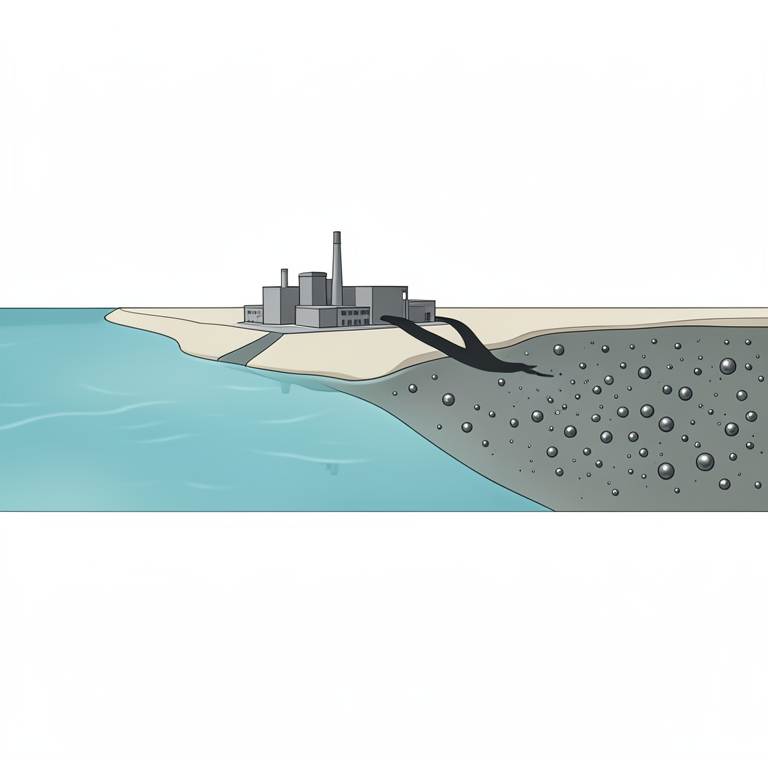
Sampling Site Comparison
AI-generated conceptual illustration (A river flowing past an industrial factory complex). It explains the idea and does not show study data.
View source evidence ↗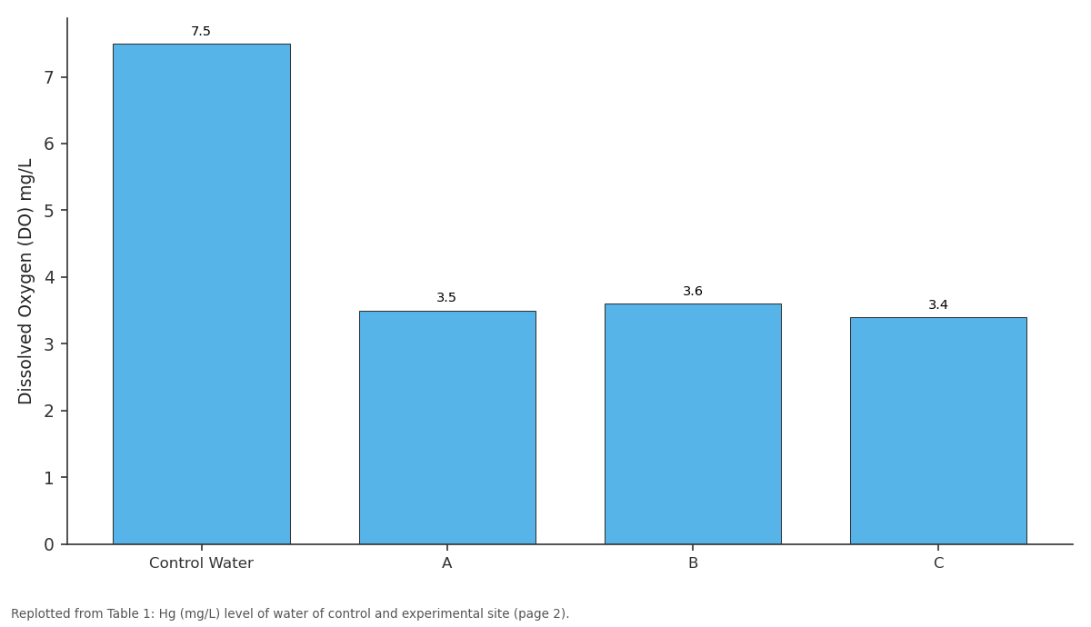
Dissolved Oxygen (DO) mg/L: Control Water vs A vs B vs C
Replotted from Table 1 (page 2) of the original paper. Every bar is the paper's own table value.
View source evidence ↗Figures & tables
From the original paper Table 1
 Table 2
 Table 2
 Table 3
 Table 4
 Table 5
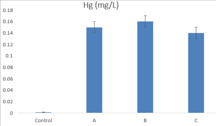 Figure 1
 Table 6
 Table 7
 Table 8
 Table 9
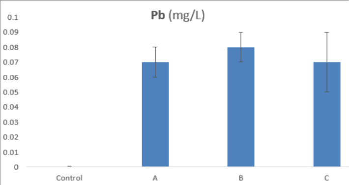 Figure 2
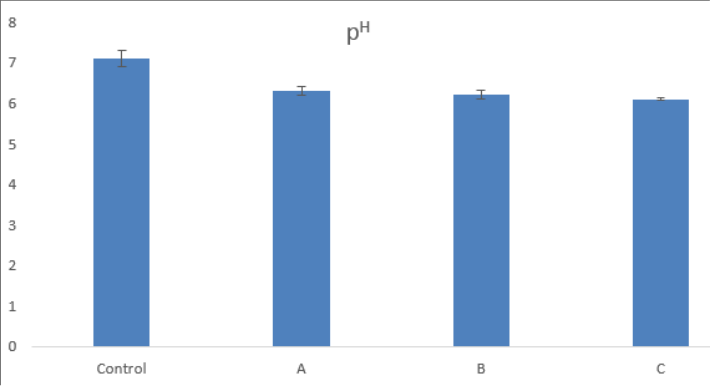 Figure 3
 Table 10
 Table 11
 Table 12
 Table 13
 Table 14
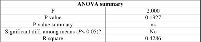 Table 15
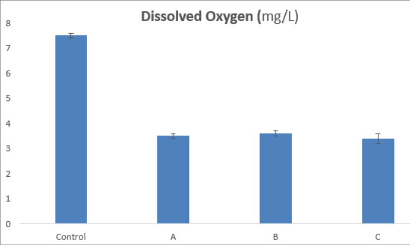 Figure 4
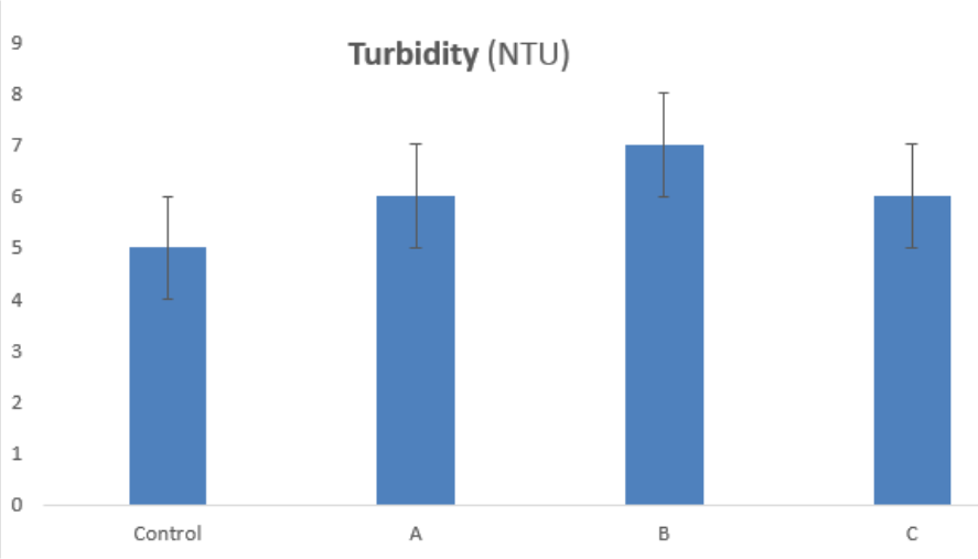 Figure 5
Introduction
Over 70% of our nation's fresh water supply that is in liquid form is rendered unfit for human use (Dwivedi, 2017) [3]. One serious environmental problem is the polluting of water by industrial waste (Johnson and Smith, 2021) [5]. Even though they are essential for economic growth, industrial operations are a major cause of water contamination (Beckerman, 1995) [1]. With an emphasis on the chemical composition, distribution, and ecological repercussions of industrial waste, this study seeks to comprehend the scope and impact of waste on water bodies.
Mercury (Hg) contamination from industrial wastewater is a growing environmental concern (Wagner-Döbler, 2003) [8]. Using field sampling, laboratory analysis, and statistical
Methods
, this research quantifies mercury concentrations in water bodies near industrial sites and assesses the ecological and health risks associated with mercury pollution (Harris et al., 2017) [4]. The objective of this research study was to determine the primary contaminants, assess their influence on human health and aquatic ecosystems, and quantify the impact of industrial waste on water quality.
Materials And Methods
2.1 Study Area The study was conducted in the industrial region of (Haldia, West Bengal, India), characterized by heavy manufacturing activities, including chemical production, metal processing, and pharmaceuticals. 2.2 Sampling Sites Water samples were collected from three sites: three near industrial discharge points (East Site-A, West Site-B, South Site-C) and one control sites located upstream (Control). 2.3 Sampling Procedure Water Samples: Collected using pre-cleaned polyethylene bottles. Sediment Samples: Taken using a grab sampler from the riverbed at each site. Biological Samples: Fish and aquatic plants were collected to assess bioaccumulation. 2.4 Laboratory Analysis Chemical Analysis: Heavy metals (Hg and Pb) were measured using atomic absorption spectroscopy (AAS) (Dalman et al., 2006) [2]. Physical Parameters: Temperature, pH, dissolved oxygen (DO), and turbidity were measured in situ using portable meters (Silva et al., 2022) [7]. IJGGE 2024; 6(1): 391-395 https://www.geojournal.net Dr. Pijush Kanti Tripathi Associate Professor, Postgraduate, Department of Geography, Haldia Government College, Haldia, West Bengal, India Dr. Pijush Kanti Tripathi Associate Professor, Postgraduate, Department of Geography, Haldia Government College, Haldia, West Bengal, India https://www.geojournal.net concentrations.
Results
2.5 Statistical Analysis Data were analyzed using ANOVA to compare pollutant levels between sites and correlation analysis to assess the relationship between industrial activities and pollutant Table 1: Hg (mg/L) level of water of control and experimental site Site Hg (mg/L) Pb (mg/L) pH Dissolved Oxygen (DO) mg/L Turbidity (NTU) Control Water 0.001 0.0005 7.1 7.5 5 A 0.15 0.07 6.3 3.5 6 B 0.16 0.08 6.2 3.6 7 C 0.14 0.07 6.1 3.4 6 Descriptive statistics Control A B C Mean 0.001333 0.1500 0.1600 0.1400 Std. Deviation 0.0005774 0.01000 0.01000 0.01000 Std. Error of Mean 0.0003333 0.005774 0.005774 0.005774 Table 2: ANOVA of Hg (mg/L) level of water of control and experimental site ANOVA table SS DF MS F (DFn, DFd) P value Treatment (between columns) 0.05033 3 0.01678 F (3, 8) = 223.4 P<0.0001 Residual (within columns) 0.0006007 8 7.508e-005 Total 0.05093 11 Table 3: Significance difference of Hg (mg/L) level of water of control and experimental site ANOVA summary F 223.4 P value <0.0001 P value summary **** Significant diff. among means (P< 0.05)? Yes R square 0.9882 Fig 1: Graphical representation of Hg (mg/L) of water of control and experimental site Table 4: Pb (mg/L) level of water of control and experimental site Descriptive statistics Control A B C Mean 0.0005000 0.07000 0.08000 0.07000 Std.
| Descriptive statistics | Control | A | B | C |
|---|---|---|---|---|
| Mean | 0.0005000 | 0.07000 | 0.08000 | 0.07000 |
| Std. Deviation | 0.0001000 | 0.01000 | 0.01000 | 0.02000 |
| Std. Error of Mean | 5.774e-005 | 0.005774 | 0.005774 | 0.01155 |
Table text extracted from the original PDF; superscript letters are shown inline. The original table image is below.
View original table image
| ANOVA summary | — |
|---|---|
| F | 223.4 |
| P value | <0.0001 |
| P value summary | **** |
| Significant diff. among means (P< 0.05)? | Yes |
| R square | 0.9882 |
Table text extracted from the original PDF; superscript letters are shown inline. The original table image is below.
View original table image
| ANOVA table | SS | DF | MS | F (DFn, DFd) | P value |
|---|---|---|---|---|---|
| Treatment (between columns) | 0.05033 | 3 | 0.01678 | F (3, 8) = 223.4 | P<0.0001 |
| Residual (within columns) | 0.0006007 | 8 | 7.508e-005 | ||
| Total | 0.05093 | 11 |
Table text extracted from the original PDF; superscript letters are shown inline. The original table image is below.
View original table image
| Descriptive statistics | Control | A | B | C |
|---|---|---|---|---|
| Mean | 0.001333 | 0.1500 | 0.1600 | 0.1400 |
| Std. Deviation | 0.0005774 | 0.01000 | 0.01000 | 0.01000 |
| Std. Error of Mean | 0.0003333 | 0.005774 | 0.005774 | 0.005774 |
Table text extracted from the original PDF; superscript letters are shown inline. The original table image is below.
View original table image
| Site | Hg (mg/L) | Pb (mg/L) | pH | Dissolved Oxygen (DO) mg/L | Turbidity (NTU) |
|---|---|---|---|---|---|
| Control Water | 0.001 | 0.0005 | 7.1 | 7.5 | 5 |
| A | 0.15 | 0.07 | 6.3 | 3.5 | 6 |
| B | 0.16 | 0.08 | 6.2 | 3.6 | 7 |
| C | 0.14 | 0.07 | 6.1 | 3.4 | 6 |
Table text extracted from the original PDF; superscript letters are shown inline. The original table image is below.
View original table image
Deviation 0.0001000 0.01000 0.01000 0.02000 Std. Error of Mean 5.774e-005 0.005774 0.005774 0.01155 Table 5: ANOVA of Pb (mg/L) level of water of control and experimental site ANOVA table SS DF MS F (DFn, DFd) P value Treatment (between columns) 0.01214 3 0.004045 F (3, 8) = 26.97 P=0.0002 Residual (within columns) 0.001200 8 0.0001500 Total 0.01334 11 https://www.geojournal.net Table 6: Significance difference of Pb (mg/L) level of water of control and experimental site ANOVA summary F 26.97 P value 0.0002 P value summary *** Significant diff. among means (P< 0.05)? Yes R square 0.9100 Fig 2: Graphical representation of Pb (mg/L) of water of control and experimental site Table 7: pH level of water of control and experimental site Descriptive statistics Control A B C Mean 7.100 6.300 6.200 6.100 Std. Deviation 0.2000 0.1000 0.1000 0.02000 Std.
| Descriptive statistics | Control | A | B | C |
|---|---|---|---|---|
| Mean | 7.100 | 6.300 | 6.200 | 6.100 |
| Std. Deviation | 0.2000 | 0.1000 | 0.1000 | 0.02000 |
| Std. Error of Mean | 0.1155 | 0.05774 | 0.05774 | 0.01155 |
Table text extracted from the original PDF; superscript letters are shown inline. The original table image is below.
View original table image
| ANOVA summary | — |
|---|---|
| F | 26.97 |
| P value | 0.0002 |
| P value summary | *** |
| Significant diff. among means (P< 0.05)? | Yes |
| R square | 0.9100 |
Table text extracted from the original PDF; superscript letters are shown inline. The original table image is below.
View original table image
| ANOVA table | SS | DF | MS | F (DFn, DFd) | P value |
|---|---|---|---|---|---|
| Treatment (between columns) | 0.01214 | 3 | 0.004045 | F (3, 8) = 26.97 | P=0.0002 |
| Residual (within columns) | 0.001200 | 8 | 0.0001500 | ||
| Total | 0.01334 | 11 |
Table text extracted from the original PDF; superscript letters are shown inline. The original table image is below.
View original table image
Error of Mean 0.1155 0.05774 0.05774 0.01155 Table 8: ANOVA of pH level of water of control and experimental site ANOVA table SS DF MS F (DFn, DFd) P value Treatment (between columns) 1.883 3 0.6275 F (3, 8) = 41.56 p<0.0001 Residual (within columns) 0.1208 8 0.01510 Total 2.003 11 Table 9: Significance difference of pH level of water of control and experimental site ANOVA summary F 41.56 P value <0.0001 P value summary **** Significant diff. among means (P< 0.05)? Yes R square 0.9397 Fig 3: Graphical representation of pH of water of control and experimental site https://www.geojournal.net Table 10: Dissolved Oxygen (mg/L) level of water of control and experimental site Descriptive statistics Control A B C Mean 7.500 3.500 3.600 3.400 Std. Deviation 0.1000 0.1000 0.1000 0.2000 Std. Error of Mean 0.05774 0.05774 0.05774 0.1155 Table 11: ANOVA of Dissolved Oxygen (mg/L) of water of control and experimental site ANOVA table SS DF MS F (DFn, DFd) P value Treatment (between columns) 36.06 3 12.02 F (3, 8) = 686.9 P<0.0001 Residual (within columns) 0.1400 8 0.01750 Total 36.20 11 Table 12: Significance difference Dissolved Oxygen (mg/L) level of water of control and experimental site ANOVA summary F 686.9 P value <0.0001 P value summary **** Significant diff. among means (P< 0.05)?
| ANOVA summary | — |
|---|---|
| F | 686.9 |
| P value | <0.0001 |
| P value summary | **** |
| Significant diff. among means (P< 0.05)? | Yes |
| R square | 0.9961 |
Table text extracted from the original PDF; superscript letters are shown inline. The original table image is below.
View original table image
| ANOVA table | SS | DF | MS | F (DFn, DFd) | P value |
|---|---|---|---|---|---|
| Treatment (between columns) | 36.06 | 3 | 12.02 | F (3, 8) = 686.9 | P<0.0001 |
| Residual (within columns) | 0.1400 | 8 | 0.01750 | ||
| Total | 36.20 | 11 |
Table text extracted from the original PDF; superscript letters are shown inline. The original table image is below.
View original table image
| Descriptive statistics | Control | A | B | C |
|---|---|---|---|---|
| Mean | 7.500 | 3.500 | 3.600 | 3.400 |
| Std. Deviation | 0.1000 | 0.1000 | 0.1000 | 0.2000 |
| Std. Error of Mean | 0.05774 | 0.05774 | 0.05774 | 0.1155 |
Table text extracted from the original PDF; superscript letters are shown inline. The original table image is below.
View original table image
| ANOVA summary | — |
|---|---|
| F | 41.56 |
| P value | <0.0001 |
| P value summary | **** |
| Significant diff. among means (P< 0.05)? | Yes |
| R square | 0.9397 |
Table text extracted from the original PDF; superscript letters are shown inline. The original table image is below.
View original table image
| ANOVA table | SS | DF | MS | F (DFn, DFd) | P value |
|---|---|---|---|---|---|
| Treatment (between columns) | 1.883 | 3 | 0.6275 | F (3, 8) = 41.56 | p<0.0001 |
| Residual (within columns) | 0.1208 | 8 | 0.01510 | ||
| Total | 2.003 | 11 |
Table text extracted from the original PDF; superscript letters are shown inline. The original table image is below.
View original table image
Yes R square 0.9961 Fig 4: Graphical representation of Dissolved Oxygen (mg/L) of water of control and experimental site Table 13: Turbidity (NTU) level of water of control and experimental site Descriptive statistics Control A B C Mean 5.000 6.000 7.000 6.000 Std. Deviation 1.000 1.000 1.000 1.000 Std. Error of Mean 0.5774 0.5774 0.5774 0.5774 Table 14: ANOVA of Turbidity (NTU) level of water of control and experimental site ANOVA table SS DF MS F (DFn, DFd) P value Treatment (between columns) 6.000 3 2.000 F (3, 8) = 2.000 P=0.1927 Residual (within columns) 8.000 8 1.000 Total 14.00 11 Table 15: Significance difference of Turbidity (NTU) level of water of control and experimental site ANOVA summary F 2.000 P value 0.1927 P value summary ns Significant diff. among means (P< 0.05)? No R square 0.4286 https://www.geojournal.net Fig 5: Graphical representation of Turbidity (NTU) of water of control and experimental site
| ANOVA summary | — |
|---|---|
| F | 2.000 |
| P value | 0.1927 |
| P value summary | ns |
| Significant diff. among means (P< 0.05)? | No |
| R square | 0.4286 |
Table text extracted from the original PDF; superscript letters are shown inline. The original table image is below.
View original table image
| ANOVA table | SS | DF | MS | F (DFn, DFd) | P value |
|---|---|---|---|---|---|
| Treatment (between columns) | 6.000 | 3 | 2.000 | F (3, 8) = 2.000 | P=0.1927 |
| Residual (within columns) | 8.000 | 8 | 1.000 | ||
| Total | 14.00 | 11 |
Table text extracted from the original PDF; superscript letters are shown inline. The original table image is below.
View original table image
| Descriptive statistics | Control | A | B | C |
|---|---|---|---|---|
| Mean | 5.000 | 6.000 | 7.000 | 6.000 |
| Std. Deviation | 1.000 | 1.000 | 1.000 | 1.000 |
| Std. Error of Mean | 0.5774 | 0.5774 | 0.5774 | 0.5774 |
Table text extracted from the original PDF; superscript letters are shown inline. The original table image is below.
View original table image
Discussion
The elevated levels of heavy metals in industrial sites are attributed to direct discharge of untreated or partially treated effluents. The data suggest significant leaching of contaminants into the water bodies, exacerbated by poor waste management practices. The high concentration of pollutants negatively affects aquatic life, as evidenced by the bioassay results. Lower pH and DO levels create a hostile environment for fish and invertebrates, disrupting ecological balance and biodiversity.
Contaminated water poses severe health risks to local communities relying on these water sources for drinking, fishing, and agriculture. Current regulatory frameworks need strengthening to enforce stricter discharge limits and promote the adoption of advanced treatment technologies. Public awareness and community engagement are crucial for sustainable waste management practices.
Conclusion
This study highlights the severe impact of industrial waste on water pollution, with significant ecological and human health implications. Immediate action is required to mitigate these effects through improved regulations, waste treatment, and community involvement.
References
8 in the original paper- Beckerman W. Economic growth and the environment: Whose growth? Whose environment? In: Growth, the Environment and the Distribution of Incomes. Edward Elgar Publishing; c1995. p. 275-290.
- Dalman Ö, Demirak A, Balcı A. Determination of heavy metals (Cd, Pb) and trace elements (Cu, Zn) in sediments and fish of the Southeastern Aegean Sea (Turkey) by atomic absorption spectrometry. Food Chem. 2006;95(1):157-162.
- Dwivedi AK. Researches in water pollution: A review. Int. Res J Nat Appl. Sci. 2017;4(1):118-142.
- Harris MJ, Stinson J, Landis WG. A Bayesian approach to integrated ecological and human health risk assessment for the South River, Virginia mercury‐contaminated site. Risk Anal. 2017;37(7):1341-1357.
- Johnson H, Smith R. Heavy Metal Pollution in Aquatic Systems. J Environ Sci. 2021;58(2):120-135.
- Madhav S, Ahamad A, Singh AK, Kushawaha J, Chauhan JS, Sharma S, et al. Water pollutants: sources and impact on the environment and human health. Sensors in water pollutants monitoring: Role of material; c2020. p. 43-62.
- Silva GME, Campos DF, Brasil JAT, Tremblay M, Mendiondo EM, Ghiglieno F, et al. Advances in technological research for online and in situ water quality monitoring: A review. Sustainability. 2022;14(9):5059.
- Wagner-Döbler I. Pilot plant for bioremediation of mercury-containing industrial wastewater. Appl. Microbiol. Biotechnol. 2003;62(2-3):124-133. 3.1 Chemical Analysis Heavy Metals: Significantly higher concentrations of Hg, Pb, and as were detected at Sites A, B, and C compared to control sites. Hg levels at Site A (0.15 mg/L), B (0.16 mg/L) and C (0.14 mg/L) exceeded the WHO limit for drinking water (0.001 mg/L). 3.2 Physical Parameters pH and DO: Lower pH (6.2) and DO levels (3.5 mg/L) were observed near industrial discharge points, indicating acidic conditions and oxygen depletion. Turbidity: Higher turbidity values were recorded at Sites A (6 NTU), B (7 NTU), and C (6 NTU), suggesting increased particulate matter from industrial runoff than control (5 NTU).
Cited by 1
From OpenAlex, OpenCitations and reference lists read by Scinovex
- Water Pollution and Contamination: Industrial, Agricultural, and Urban Impacts ↗
Sylvester Chibueze Izah, Matthew Chidozie Ogwu · Springer water · 2026
❝ 13