
Research article · 2024 · Full text
International Journal of Research in AgronomyModelling potential evapotranspiration: Statistical analysis for Madurai’s water dynamics
Volume 7(7S) · Pages 194–200 · DOI: 10.33545/2618060x.2024.v7.i7sc.1009 ↗
Research areasWater resources management and optimization
Abstract
Author-writtenPotential evapotranspiration is a comprehensive process encompassing both evaporation and transpiration that helps to determine the removal of water from both the soil and plant surfaces. It serves as a crucial mechanism for returning moisture to the atmosphere. The study specifically concentrates on computing the Weekly Potential Evapotranspiration (PET) for Madurai district. Models such as FAO Penman-Monteith, Modified Penman, Penman, Priestley Taylor, Blaney Criddle and Hargreaves models were compared in this study using Multiple Linear Regression. Performance of the fitted models were compared using accuracy metrics such as Root Mean Squared Error (RMSE), RAE, Mean Absolute Error (MAE), Mean Absolute Percentage Error (MAPE), and the coefficient of determination (R2). The Penman model emerged as the most pertinent model, exhibiting the least bias and the highest R2.
Summary
Source-checkedPlain-language reading of the full paper, prepared with AI and checked against the text. Each point links to the authors' own words.
Why it matters
- Potential evapotranspiration (PET) is critical for managing agricultural production, irrigation, and assessing droughts and hydrological processes. View evidence ↗
- Calculating PET allows for a precise understanding of crop water demand, which helps prevent water waste in farming. View evidence ↗
- Estimating PET depends on meteorological data, including temperature, rainfall, wind speed, sunshine hours, relative humidity, and extra-terrestrial radiation. View evidence ↗
The question
- The study aims to determine weekly PET for the Madurai district using six empirical models and identify the best-fitted model via Multiple Linear Regression (MLR) to predict future values. View evidence ↗
What they did
- The research used secondary meteorological data from 2020 for the Madurai district in Tamil Nadu, India, sourced from the Agro Climate Research Centre. View evidence ↗
- Six empirical models were compared using MLR: FAO Penman-Monteith, Modified Penman, Penman, Priestley Taylor, Blaney Criddle, and Hargreaves. View evidence ↗
- The researchers used R-Software to split the dataset into an 80% training set and a 20% testing set. View evidence ↗
- Model effectiveness was evaluated using accuracy metrics including RMSE, RSE, MAE, and MAPE. View evidence ↗
What they found
- Following the Penman model, the Hargreaves and FAO PM models were the next most relevant, both showing an R2 of 0.97. View evidence ↗
- The Priestley Taylor (PT) model did not perform well with the dataset provided. View evidence ↗
- Correlation analysis revealed a notable relationship (0.78) between minimum temperature and minimum relative humidity. View evidence ↗
- Extra-terrestrial radiation (Ra) showed high correlations with net radiation (Rn) at 0.77 and maximum temperature (Tmax) at 0.90. View evidence ↗
What it means
- The authors conclude that the estimated PET values from these empirical models can be used to determine crop water requirements for farmers in the Madurai district. View evidence ↗
Visual summary
3 visualsIllustrations explain the paper; charts are replotted from the paper's own table values.
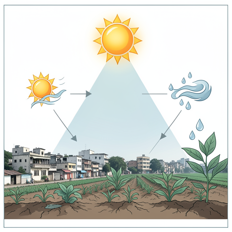
Model Comparison Hierarchy
AI-generated conceptual illustration (A landscape of Madurai, India, featuring urban buildings and agricultural fields under a bright sun). It explains the idea and does not show study data.
View source evidence ↗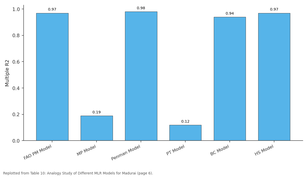
Multiple R2: FAO PM Model vs MP Model vs Penman Model vs PT Model vs BC Model
Replotted from Table 10 (page 6) of the original paper. Every bar is the paper's own table value.
View source evidence ↗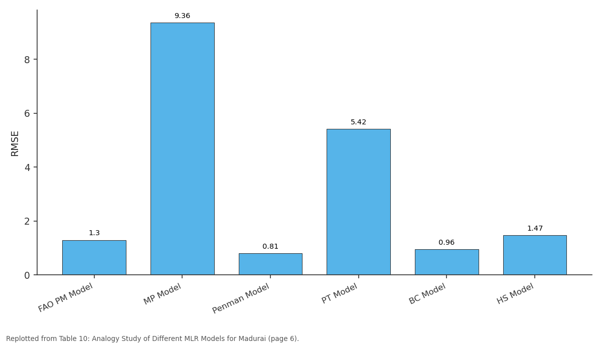
RMSE: FAO PM Model vs MP Model vs Penman Model vs PT Model vs BC Model
Replotted from Table 10 (page 6) of the original paper. Every bar is the paper's own table value.
View source evidence ↗Figures & tables
From the original paper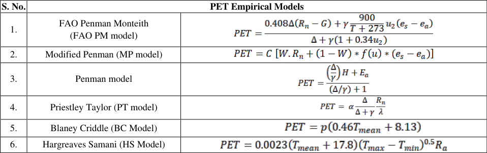 Table 1
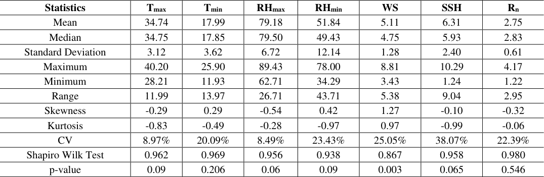 Table 2
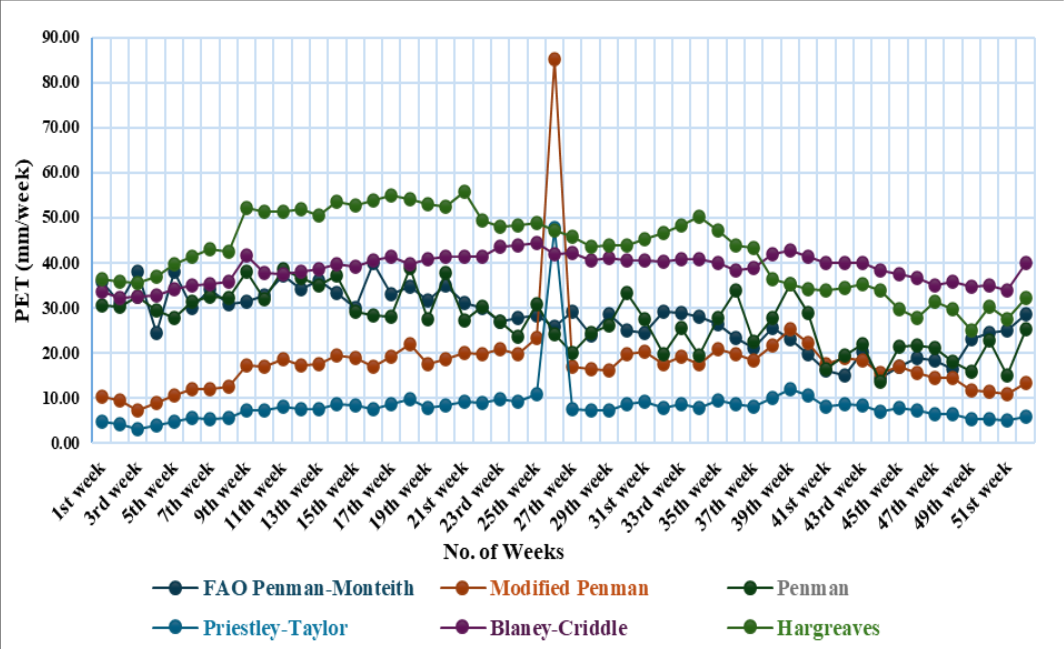 Figure 1
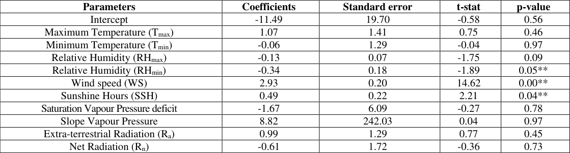 Table 3
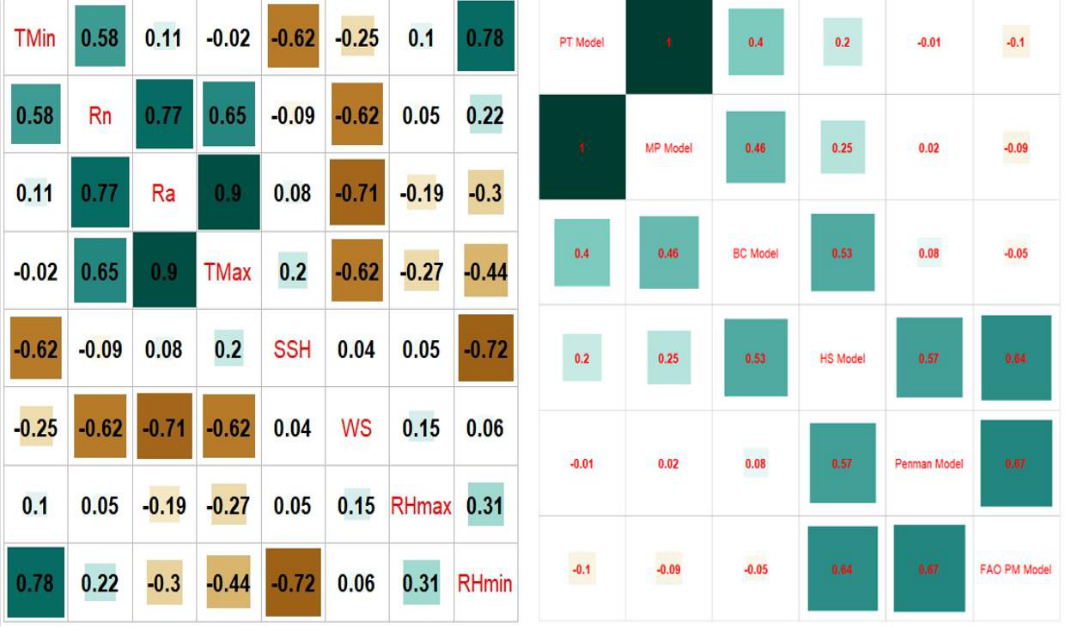 Figure 2
 Table 4
 Table 5
 Table 6
 Table 7
 Table 8
 Table 10
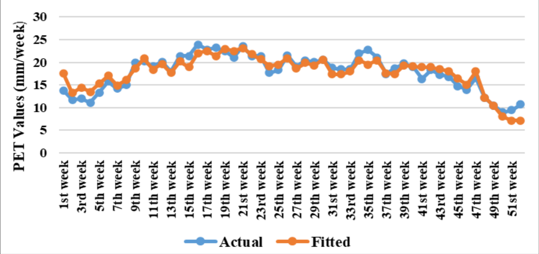 Figure 6
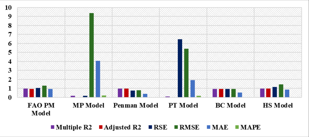 Figure 5
Introduction
Potential evapotranspiration holds significant importance in ecological, hydrological, and drought assessment processes, as well as in the management of agricultural production and irrigation. Its pivotal role extends to influencing hydrological processes, determining water requirements for crops, impacting crop production, and guiding irrigation management practices (Djaman et al. 2018) [6] . The calculation of potential evapotranspiration enables a precise understanding of the water demand for crops at specific times and intervals, thereby preventing unnecessary water wastage in agricultural fields. This estimation relies on key meteorological parameters such as temperature, rainfall, relative humidity, wind speed, sunshine hours, and extra-terrestrial radiation (Sriram and Rashmi. 2014) [21] . By taking into account these factors, the calculation of potential evapotranspiration becomes instrumental not only in the efficient management of water resources but also in optimizing nutrient movement within plants and enhancing plant temperature. This parameter assumes a pivotal role in the hydrologic budget and precipitation, serving as a linchpin in maintaining ecological balance and bolstering agricultural productivity. Moreover, potential evapotranspiration plays a critical role in determining the water requirements of crops, facilitating the regulation of water amounts provided to farmers and influencing the design of irrigation schemes (Droogers and Allen 2002) [8] . Various methods, including Lysimeter experiments, water budget analyses, energy balance assessments, field experiments, and open pan evaporimeters, are employed to calculate potential evapotranspiration (Hajare et al. 2008) [11] . Recent technological advancements have introduced the application of remote sensing and Geographic Information System (GIS) for estimating potential evapotranspiration, although these methods may not be directly applicable for field measurements. Empirical models, widely utilized, offer an alternative approach for computing potential evapotranspiration. The determination of water requirements in irrigated areas relies on consumptive use, taking into account monthly temperature, sunshine hours, and the irrigating season, as proposed by Blaney and Criddle in 1950 [4] . Fennessey and Vogel (1996) [9] developed multivariate models based on reference crop evapotranspiration and pan evaporation. Xu and Singh (2000) [22] utilized radiation-based methods to calculate evaporation. Saikia et al. (2005) [19] identified the most suitable model for potential evapotranspiration (PET) and pan evaporation through multiple linear regression (MLR) and correlation analysis. Alkaeed et al. (2006) [1] evaluated reference evapotranspiration on a monthly basis, correlating solar radiation-based models and net radiationbased models with FAO Penman Monteith model. Gavilan (2006) [10] compared Hargreaves' model with FAO Penman Monteith across 86 meteorological stations. Chowdhury et al. (2010) [5] validated the PET model with pan-derived evapotranspiration. Liu et al. (2013) [14] employed regression analysis to identify relevant models by comparing them with empirical models. Rajasekhar et al. (2015) [23] assessed the closeness of the FAO Penman Monteith model to other empirical models. Helder et al. (2016) [13] compared the FAO Penman Monteith model with other models using multiple linear regression. Sharafi and Galeni (2021) [18] evaluated multivariate linear regression for reference evapotranspiration. Archana et al. (2021) [3] focused on predicting potential evapotranspiration on a weekly basis. The study's objective is to determine weekly potential evapotranspiration for Madurai using six empirical models and predict PET values for future weeks based on the best-fitted model using MLR and performance metrics.
Materials and methods
The investigation was carried out in Madurai, a district located in Tamil Nadu, India, nestled within the Eastern Ghats. Positioned at a latitude of 9.93° North and a longitude of 78.12° East, the city maintains an average elevation of 101 meters. The study relied on secondary data obtained from the Agro Climate Research Centre at Tamil Nadu Agricultural University in Coimbatore, covering the period of 2020. The dataset comprises crucial parameters such as maximum temperature, minimum temperature, maximum relative humidity, minimum relative humidity, rainfall, extra-terrestrial radiation, wind speed, and sunshine hours for the specific location of Madurai.
Correlation Analysis
Correlation measures the association between predicted and predictor variables. By quantifying the strength and direction of the relationship between two variables. The correlation coefficient ranges from 0 to 1, where 0 indicates no correlation or a completely random relationship, and 1 signifies a perfect positive correlation (Shankar et al., 2022) [20] . This numerical scale provides insights into the degree to which changes in one variable correspond to changes in another, offering a valuable tool in understanding and assessing statistical associations.
Empirical models
The focus of this study is on six distinct empirical models utilized for deriving Potential Evapotranspiration (PET) values from various covariates. The FAO Penman-Monteith model, formulated by Howard Latimer Penman and John Monteith, is widely recognized as the standard model for evaluating PET (Allen et al., 1998) [2] . However, the Modified Penman model tends to overestimate PET, even in conditions of high wind and low evaporation (Doorenbos and Pruitt, 1977) [7] . H. L. Penman (1948) [16] proposed the Penman Model, a combination of aerodynamics and heat balance methods. Additionally, Potential Evapotranspiration can be estimated using temperature-based methods such as Hargreaves Samani (1982) [12] . The mathematical descriptions of these models are provided in Table 1.
| S. No. | PET Empirical Models | — |
|---|---|---|
| 1. | FAO Penman Monteith (FAO PM model) | |
| 2. | Modified Penman (MP model) | |
| 3. | Penman model | |
| 4. | Priestley Taylor (PT model) | |
| 5. | Blaney Criddle (BC Model) | |
| 6. | Hargreaves Samani (HS Model) |
Table text extracted from the original PDF; superscript letters are shown inline. The original table image is below.
View original table image
Results and Discussions
In this research paper, the potential evapotranspiration was estimated using six different models for Madurai. Using the standard meteorological week's table, the daily PET converted into weekly PET value by taking averages. The PET value is estimated using the different models were given in the Fig 1.
Among these models, FAO Penman-Monteith model considered a standard model for estimating the potential evapotranspiration. The partial regression coefficients of the independent variables and the error term are shown in the following Table 3. Each of the coefficients was interpreted as the estimated change in FAO Penman-Monteith PET values for each of the variables. The significance of the results was determined by interpreting P values of the regression results that were less than 0.05 in value. MP Model were built between PET value of Modified Penman and the independent variable as , , f(U), ( ), and . The mean temperature and relative humidity was considerable at statistically significant at 5% respectively which displayed in Table 4. PT Model were analysed using the predicted variable as evaluated Priestley-Taylor PET values and predictor variable as mean temperature (
| Parameters | Coefficients | Standard error | t-stat | p-value |
|---|---|---|---|---|
| Intercept | 104.64 | 264.07 | 0.39 | 0.69 |
| Mean Temperature (TMean) | 11.33 | 15.02 | 0.76 | 0.04** |
| Relative Humidity (RHMean) | 0.27 | 0.34 | 0.82 | 0.04** |
| Wind speed (f(U) | -707.61 | 753.75 | -0.94 | 0.35 |
| Slope Vapour Pressure | -954.13 | 1419.96 | -0.67 | 0.51 |
| Net Radiation (Rn) | -2.37 | 6.80 | -0.35 | 0.73 |
Table text extracted from the original PDF; superscript letters are shown inline. The original table image is below.
View original table image
), slope vapour pressure (Δ), and net radiation ( ) were shown in table 6. The mean temperature was considered as significant variables in the PT Model. The Model were built in the form as given below, Y PT Model = -40.93 + 5.06 T mean -411.47 ∆ + 0.02 R n BC Model were built between Blaney-Criddle PET value as the regressand and regressors as , and p. Table 7 showed that the mean temperature and daily percentage were considered as the significant variables.
| Parameters | Coefficients | Standard error | t-stat | P Value |
|---|---|---|---|---|
| Intercept | -20.19 | 4.31 | -4.69 | 0.00** |
| Mean Temperature (T ) mean | 0.85 | 0.07 | 11.69 | 0.00** |
| Mean Daily Percentage (p) | 133.97 | 19.37 | 6.92 | 0.00** |
Table text extracted from the original PDF; superscript letters are shown inline. The original table image is below.
View original table image
| Parameters | Coefficients | Standard error | t-stat | p-value |
|---|---|---|---|---|
| Intercept | -40.93 | 50.69 | -0.81 | 0.43 |
| Mean Temperature (Tmean) | 5.06 | 7.46 | 0.68 | 0.00** |
| Slope Vapour Pressure | -411.47 | 711.99 | -0.58 | 0.57 |
| Net Radiation (Rn) | 0.02 | 3.38 | 0.01 | 0.99 |
Table text extracted from the original PDF; superscript letters are shown inline. The original table image is below.
View original table image
Y BC Model = -20.19 + 0.85 T mean + 133.97 p
Selection criteria
The accuracy of the model tested using RMSE, RSE, MAE, MAPE, R 2 and Adj R 2 . The Penman model considered as a relevant model which shows the maximum coefficient of determination (0.98) and minimum RMSE (0.81), RSE (0.77), MAE (0.39) and MAPE (1.47%) values. Next to the Penman model, Hargreaves model and FAO PM Model was observed with highest R 2 (0.97) and least error values. PT models fails to perform well for the given data.
Conclusion
In this study, the Potential evapotranspiration was estimated using six different empirical models for Madurai district which can be utilized to determine the crop water requirement for the farmers. The estimated PET value intrepreted that the highest PET value indicates the influence of temperature and relative
Figures and tables from the paper
| Statistics | T max | T min | RH max | RH min | WS | SSH | R n |
|---|---|---|---|---|---|---|---|
| Mean | 34.74 | 17.99 | 79.18 | 51.84 | 5.11 | 6.31 | 2.75 |
| Median | 34.75 | 17.85 | 79.50 | 49.43 | 4.75 | 5.93 | 2.83 |
| Standard Deviation | 3.12 | 3.62 | 6.72 | 12.14 | 1.28 | 2.40 | 0.61 |
| Maximum | 40.20 | 25.90 | 89.43 | 78.00 | 8.81 | 10.29 | 4.17 |
| Minimum | 28.21 | 11.93 | 62.71 | 34.29 | 3.43 | 1.24 | 1.22 |
| Range | 11.99 | 13.97 | 26.71 | 43.71 | 5.38 | 9.04 | 2.95 |
| Skewness | -0.29 | 0.29 | -0.54 | 0.42 | 1.27 | -0.10 | -0.32 |
| Kurtosis | -0.83 | -0.49 | -0.28 | -0.97 | 0.97 | -0.99 | -0.06 |
| CV | 8.97% | 20.09% | 8.49% | 23.43% | 25.05% | 38.07% | 22.39% |
| Shapiro Wilk Test | 0.962 | 0.969 | 0.956 | 0.938 | 0.867 | 0.958 | 0.980 |
| p-value | 0.09 | 0.206 | 0.06 | 0.09 | 0.003 | 0.065 | 0.546 |
Table text extracted from the original PDF; superscript letters are shown inline. The original table image is below.
View original table image
| Parameters | Coefficients | Standard error | t-stat | p-value |
|---|---|---|---|---|
| Intercept | -8.24 | 12.28 | -0.67 | 0.51 |
| Mean Temperature (Tmean) | 0.77 | 1.33 | 0.58 | 0.57 |
| Relative Humidity (RHmean) | -0.02 | 0.04 | -0.67 | 0.51 |
| Wind speed (WS) | -0.19 | 0.14 | -1.35 | 0.02** |
| Slope Vapour Pressure | -46.48 | 118.73 | -0.39 | 0.69 |
| Flux density of sensible heat to air (H) | 5.39 | 0.22 | 24.61 | 0.00** |
| Saturated Vapour Pressure (Ea) | 0.08 | 0.87 | 0.09 | 0.93 |
| Net Radiation (Rn) | 0.03 | 0.77 | 0.04 | 0.97 |
Table text extracted from the original PDF; superscript letters are shown inline. The original table image is below.
View original table image
| S. No. | Model | Multiple R2 | Adjusted R2 | RSE | RMSE | MAE | MAPE |
|---|---|---|---|---|---|---|---|
| 1. | FAO PM Model | 0.97 | 0.96 | 1.04 | 1.30 | 0.93 | 3.85% |
| 2. | MP Model | 0.19 | 0.04 | 0.19 | 9.36 | 4.08 | 20.08% |
| 3. | Penman Model | 0.98 | 0.98 | 0.77 | 0.81 | 0.39 | 1.47% |
| 4. | PT Model | 0.12 | 0.02 | 6.46 | 5.42 | 1.93 | 17.92% |
| 5. | BC Model | 0.94 | 0.93 | 0.93 | 0.96 | 0.55 | 1.90% |
| 6. | HS Model | 0.97 | 0.97 | 1.16 | 1.47 | 0.87 | 2.41% |
Table text extracted from the original PDF; superscript letters are shown inline. The original table image is below.
View original table image
References
22 in the original paper- Alkaeed O, Flores C, Jinno K, Tsutsumi A. Comparison of several reference evapotranspiration methods for Itoshima Peninsula area, Fukuoka, Japan. Memoirs of the Faculty of Engineering, Kyushu University. 2006;66:1-14.
- Archana A, Radha M, Dheebhakaran GA, Vanitha G. Assessment and comparison of potential evapotranspiration for the district of Coimbatore using statistical modelling approach. The Pharma Innovation Journal. 2021;SP10(10):530-539.
- Blaney HF, Criddle WB. Determining water requirements in irrigated areas from climatological and irrigation data. USDA Agricultural SCS-TP. 1950;96.
- Chowdhury S, Nanda MK, Saha G, Deka N. Evaluation of different methods for evapotranspiration estimation using automatic weather station data. Journal of Agrometeorology. 2010;12(1):85-88.
- Djaman K, O'Neill M, Owen CK, Smeal D, Koudahe K, West M, Allen S, Lombard K, Irmak S. Crop evapotranspiration, irrigation water requirement and water productivity of maize from meteorological data under semiarid climate. Water. 2018;10:405.
- Doorenbos J, Pruitt WO. Guidelines for predicting crop water requirements. FAO Irrigation and Drainage Paper 24. FAO, Rome, Italy. 1977.
- Droogers P, Allen RG. Estimating reference evapotranspiration under inaccurate data conditions. Irrigation Science. 2002;16:33-45.
- Fennessey NM, Vogel RM. Regional models of potential evaporation and reference evapotranspiration for the northeast USA. Journal of Hydrology. 1996;184(3-4):337354.
- Gavilan P, Lorite IJ, Tornero S, Berengena J. Regional calibration of Hargreaves equation for estimating reference evapotranspiration in a semiarid environment. Agricultural Water Management. 2006;81:257-281.
- Hajare HV, Raman NS, Dharkar JM. New technique for evaluation of crop water requirement. WSEAS Transactions on Environment and Development. 2008;4(5):436-446.
- Hargreaves GH, Samani A. Estimating potential evapotranspiration. Journal of the Irrigation and Drainage Division, Proceedings of the American Society of Civil Engineers. 1982;108(IR3):225-230.
- Helder JF da Silva, Marconio S, dos Santo, Jório B Cabral Junior, Maria HC, Spyrides. Modeling of reference evapotranspiration by multiple linear regression. Journal of Hyperspectral Remote Sensing. 2015;6:44-58.
- Liu H, Li Y, Zhang R, Huang G. Evaluation and modification of potential evapotranspiration methods in Beijing, China. International Journals of Agriculture and Biological Engineering. 2013;6(4).
- Penman HL. Estimating evapotranspiration. Transactions of the American Geophysical Union. 1956;37:43-46.
- Penman HL. Natural evaporation from open water, bare soil and grass. Proceedings of the Royal Society of London, Series A. 1948;193:120-146.
- Priestley CHB, Taylor RJ. On the assessment of the surface heat flux and evaporation using large-scale parameters. Monthly Weather Review. 1972;100:81-92.
- Sharafi S, Galeni MM. Evaluation of multivariate linear regression for reference evapotranspiration modeling in different climates of Iran. Theoretical and Applied Climatology. 2021;143:1409-1423.
- Saikia US, Satapathy KK, Goswami B, Lama TD. Estimation of PET by empirical models for northeastern hill region of Meghalaya. Journal of Agrometeorology. 2005;7(2):268-273.
- Shankar SV, Ajaykumar R, Prabhakaran P, Kumaraperumal R, Guna M. Modelling of tea mosquito bug (Helopeltis theivora) incidence on neem tree: A zero inflated count data analysis. Journal of Agrometeorology. 2022;24(4):409-16.
- Sriram AV, Rashmi CN. Estimation of potential evapotranspiration by multiple linear regression method. IOSR Journal of Mechanical and Civil Engineering. 2014;11(2):65-70.
- Xu C-Y, Singh VP. Evaluation and generalization of radiation-based methods for calculating evaporation. Hydrological Processes. 2000;14:339-349.
- Rajasekhar K, Suresh SN, Manjithaya R, Govindaraju T. Rationally designed peptidomimetic modulators of Aβ toxicity in Alzheimer's disease. Scientific reports. 2015 Jan 30;5(1):8139.
Cited by 1
From OpenAlex, OpenCitations and reference lists read by Scinovex
- Assessment of maize evapotranspiration, water requirements and productivity using weather data in Coimbatore’s semiarid climate ↗
M Raguramakrishnan, S Pazhanivelan, M Raju, Ramalingam Kumaraperumal, Kavitha Ravi, A. Senthil · Plant Science Today · 2024
Accurately estimating crop water use is crucial for efficient water management in conservation agriculture, especially in Coimbatore's semiarid climate. This study assessed maize water use and productivity over three growing seasons (2023-2024) at AC&RI, Coimbatore. Irrigation applied each season varied between 500.8mm and 554.1 mm, averaging 535.8 mm, while total water supply ranged from 810.6 to 985.3 mm. Actual evapotranspiration…
❝ 0PDF