
Research article · 2024 · Full text
International Journal of Research in AgronomyAssessment of above-ground biomass carbon using optical and microwave remote sensing data
Volume 7(7S) · Pages 102–108 · DOI: 10.33545/2618060x.2024.v7.i7sb.1003 ↗
Research areasAtmospheric and Environmental Gas DynamicsOil, Gas, and Environmental Issues
Abstract
Author-writtenForests are nature’s most attractive and versatile renewable resources, providing a wide range of social, economic, environmental services and benefits. The modeling of carbon balance depends heavily on forests, as they are considered as carbon reservoir. Accurate measurements of biomass and other forest bio physical parameters are necessary to better understand the global carbon cycle. Remote sensing (RS) based AGB estimation approaches have become increasingly popular as non-destructive means of biomass estimation but constitute limited applications, since the green felling in natural forests and plantations is prohibited. The primary sources for AGB estimation are optical data, radio detection and ranging (RADAR) and light detection and ranging (LIDAR) systems. In this context the study was carried out in the Dubare forest of moist deciduous vegetation type of Kushalnagar taluk, Kodagu district to assess the above-ground biomass carbon using optical and microwave remote sensing data. Totally 25 field sampling plots were randomly used for field data collection. Previously developed relevant allometric equations were used to estimate above- ground tree biomass (AGTB) using GBH and height in each plot. The results revealed that the AGTB ranged from 129.05 Mg ha-1 to 355.54 Mg ha-1, total carbon stocks ranged from 60.65 Mg ha-1 to 167.11 Mg ha-1, while CO2e was found to be ranging from 222.4 Mg ha-1 to 612.7 Mg ha-1. The regression model obtained between above-ground tree biomass and Synthetic Aperture Radar (SAR) backscatter value performed well with VH polarization than VV polarization with an R2 value of 0.69 and RMSE of 31.87 Mg ha-1. The best fit regression model was obtained between above-ground tree biomass and Normalized Difference Vegetation Index (NDVI) with the highest R2 value of 0.75 and a low RMSE value of 28.20 Mg ha-1.
Summary
Source-checkedPlain-language reading of the full paper, prepared with AI and checked against the text. Each point links to the authors' own words.
Why it matters
- Forests serve as critical carbon reservoirs and provide essential social, economic, and environmental services, making them central to carbon balance modeling. View evidence ↗
- Precise measurements of forest biomass and biophysical parameters are necessary to understand global warming and the global carbon cycle. View evidence ↗
- While optical remote sensing is useful, microwave remote sensing is superior in areas with heavy cloud cover because it can penetrate clouds and vegetation in all weather and lighting conditions. View evidence ↗
The question
- The study aimed to assess above-ground biomass carbon in the moist deciduous Dubare forest of Kodagu district using both optical and microwave remote sensing data. View evidence ↗
What they did
- The researchers used a random sampling method consisting of five 100m x 100m super plots, each containing five 20m x 20m main plots (at the corners and center) to assess biomass. View evidence ↗
- Field data collection included GPS coordinates, species identification, and the height and girth (for trees ≥30cm) of trees in each plot. View evidence ↗
- Regression models for predicting above-ground biomass (AGB) were developed using Sentinel-1A (SAR) and Sentinel-2A (optical) satellite data processed with SNAP and ArcGIS software. View evidence ↗
What they found
- Field measurements showed that above-ground tree biomass (AGTB) ranged from 129.05 to 355.54 Mg ha-1, carbon stocks from 60.65 to 167.11 Mg ha-1, and CO2 equivalent from 222.4 to 612.7 Mg ha-1. View evidence ↗
What it means
- The authors concluded that the optical remote sensing model is the most accurate method for estimating above-ground tree biomass in this study. View evidence ↗
- The authors suggest that integrating multisource data, combining optical and microwave data from various resolutions (e.g., SAR, Landsat, LIDAR), could improve the precision of global AGB estimation. View evidence ↗
- Discrepancies between projected and observed biomass may be caused by variations in tree phenological states and crown density. View evidence ↗
Visual summary
1 visualsIllustrations explain the paper; they do not show study data.
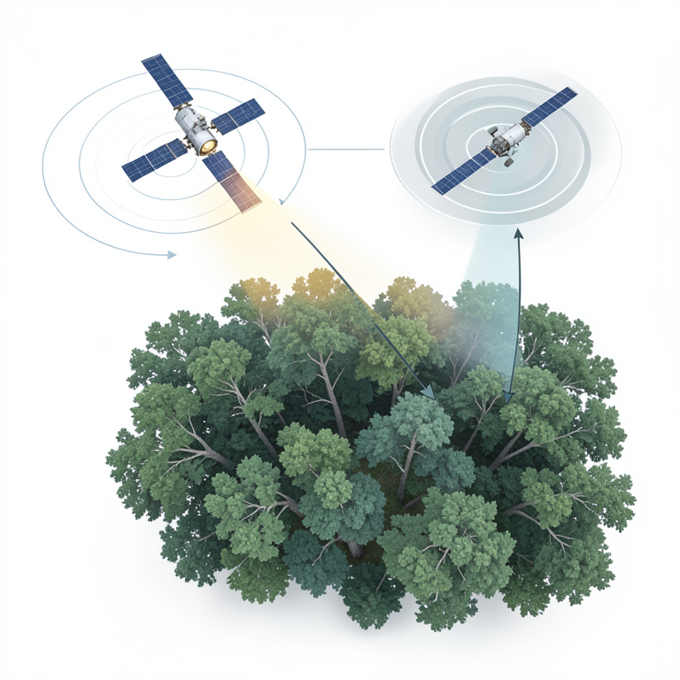
Remote Sensing Data Comparison
AI-generated conceptual illustration (temperate forest canopy and two satellites). It explains the idea and does not show study data.
View source evidence ↗Figures & tables
From the original paper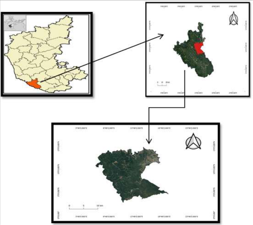 Figure 1
 Table 1
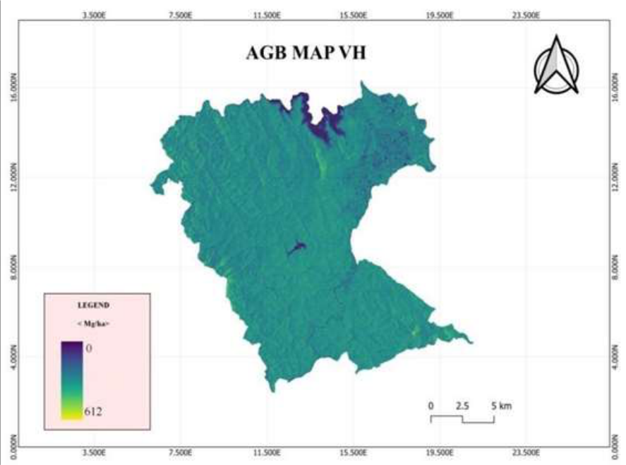 Figure 2
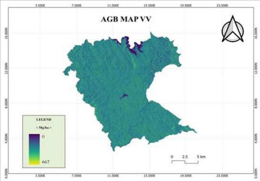 Figure 3
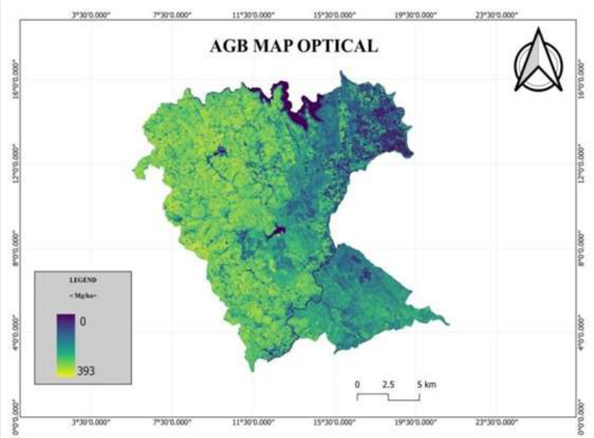 Figure 4
Introduction
Forests are nature's attractive and versatile renewable resources, providing a wide range of social, economic, cultural and environmental services. Forests play a significant part in creating a healthy ecosystem and reducing environmental pollutants. In India, forests cover almost 21.71 percent of the country's total land area (Singh et al., 2021) [35] . Forests play an important role in regional and global carbon cycles as they store large quantities of carbon in vegetation and soil. Around 80 percent of the world's terrestrial above-ground carbon stores (biomass) are found in forests, which also play a significant role in the global carbon cycle. The measurement of biomass and subsequent carbon is currently a key part of the REDD+ projects. REDD+ is a set of finance instruments and incentives designed to slow down deforestation and forest degradation in order to combat climate change. Due to deforestation, carbon dioxide, more greenhouse gases remain in the atmosphere. Therefore, accurate measurements of biomass and other forest biophysical parameters are essential for better understand the global carbon cycle and global warming. Biomass estimation is done by using a destructive method and a non-destructive method. A non-destructive method is mainly based on regression equations which are derived from measurable tree parameters like diameter at breast height (dbh), basal area and tree height.
There is a need for global, high temporal resolution forest biomass monitoring techniques, possibly using remote sensing. Optical remote sensing has been successful in forest biomass studies but over limited geographical regions. In areas where cloud cover problem is predominant, it could not be really used. In these conditions, microwave remote sensing provides the best solution as it has several advantages over optical remote sensing in all weather, day and night conditions, penetration through clouds, vegetation, dry soil, sand and dry snow. It is sensitive to surface roughness, dielectric properties, moisture content, polarization, frequency and imaging possibility from different types of polarized energy (HH, VV, HV, and VH). By the late 1970s and 1980s Synthetic aperture radar (SAR) remote sensing emerged as a solution to the limitations faced by traditional optical sensors. SAR sensors on account of their much longer wavelengths (1 mm to 1m) have not only cloud penetrating capability but also the waves can penetrate the atmospheric moisture as well as the upper vegetation layer of the forest canopy and waves are scattered by leaves, twigs, branches and stem. In this context, the present study aimed at using optical and SAR data to assess and model the forest above-ground biomass.
Materials and Methods
Materials and Methods
Study area
The study was carried out in the moist deciduous forest of Kushalnagar taluk, Kodagu district, in the Central Western Ghats of Karnataka. The Kodagu district lies between 11° 56' and 12° 52' N at Northern latitudes and Eastern longitudes of 72° 22' and 76° 12' E. The study area has a tropical humid environment, the elevation ranges from 50 to 1750 m above sea level (MSL), with rainfall ranging from 1500 to 3500 mm in a year.
Development of spectral model and AGB Mapping Satellite data:
The establishment of the Regression equation model for predicting AGB was done using Sentinel-1A of SAR data and Sentinel-2A of optical data of the same area using SNAP and ArcGIS software.
Regression analysis: Regression analysis is a set of statistical methods used for the estimation of relationships between a dependent variable and independent variables. Assessing the strength of the relationship between variables and for modelling the future relationship between them. The basic concept of regression analysis involves fitting a regression model to a set of data points and estimating the parameters that define the relationship between the variables. The dependent variable, also known as the response variable or outcome variable, is the variable that is being predicted or explained. The independent variables, also known as predictor variables or explanatory variables, are the variables that are believed to influence or explain the variation in the dependent variable.
Linear regression equation model:
It attempts to model the relationship between two or more explanatory variables and a response variable by fitting a linear equation to observed data. Every value of the independent variable x is associated with a value of the dependent variable y.
Using the data analysis toolpak, creating a regression output in excel is followed by the steps mentioned here. By selecting data from the toolbar. The data menu displays the data analysisanalysis tools dialog box displays. From the menu, by selecting regression, in the regression dialog box select the dependent variable data(biomass) in the input Y range. In the input X range select the independent variable data (NDVI value or HH, HV polarisation value). The obtained intercept was used to establish the regression equation. The NDVI was calculated using the formula given by Jensen (2000) [39] .
The equation was validated using ground truth data of 25 plots. The RMSE and R 2 were used to evaluate the equation (Anup et al., 2016) [3] .
Results and Discussion
The above-ground biomass and carbon stock of the forest were estimated using plot-wise volume calculations. After estimating the volume calculations of all plots, the above-ground tree biomass of the forest and the total quantity of carbon sequestered for the moist deciduous forest of the Kushalnagar taluk, Kodagu district were estimated. The following result of experiments on above-ground tree biomass and carbon stock are presented
Assessment of AGTB using optical data
The results of the present study revealed that out of the total 25 plots, the ground-based volume observed in the study area ranging from 234.85 m 3 ha -1 to 517.81 m 3 ha -1 . Similarly, aboveground tree biomass was observed in the study area, which varied between 129.05 Mg ha -1 and 355.54 Mg ha -1 . A variation in the number of trees, their height, and gbh was attributed for the variation in above-ground tree biomass and volume.
The carbon stock in the study area ranged from 60.65 Mg ha -1 to 167.11 Mg ha -1 and the area's total carbon dioxide equivalent (CO2e) was found to be 222. [15] . Most microwave sensors produce signals that are either horizontally or vertically polarised. Longer wavelengths (L and P band) with VV and VH polarisations have been shown to produce better results than short wavelengths. The results of the current study revealed that SAR backscatter values ranged from -10.87 dB to -21.74 dB, while the predicted above-ground tree biomass ranged from 143.63 Mg ha -1 to 348.68 Mg ha -1 for VH polarisation.
Similarly, SAR backscatter values with VV polarisation ranged from -6.81 dB to -18.12 dB and predicted above-ground tree biomass values ranged from 143.63 Mg ha -1 to 348.68 Mg ha -1 .
The results differ because they rely on signal saturation, which is a function of wavelength, polarization and the characteristics of the vegetation cover which is also associated with roughness, geometry, dielectric properties as well as of the difficulties caused by the specific properties of the ground such as slope and aspect.
Development of spectral model and AGB Mapping Regression equation model for above-ground biomass with backscatters of SAR data
The regression (Linear) model was obtained between aboveground tree biomass and SAR backscatter values in the study area. The VH polarisation had an R 2 value of 0.69, which was best and followed by the VV polarisation with the lowest R 2 value of 0.65. VV polarisation had a higher RMSE value at 33.87 Mg ha -1 , while VH polarisation had 31.87 Mg ha -1 . The linear regression equation is validated with 25 plots of ground truth data which shows a percent difference of biomass values from -20.20% to 69.43% in the VH polarisation followed by -27.31% to 22.84% in VV polarisation. The model is most suitable for VH polarisation followed by VV polarisation. The direct relationship between microwave backscatter values and plot-wise above-ground tree biomass was observed comparatively low due to variation in errors present in the high biomass region i.e., >200 t/ha. This could be attributed to two types of uncertainties, 1) the exclusion of small trees (< 30 cm) GBH and 2) the saturation of SAR signal at high biomass regions and topographic effects of the study area. The polarimetric-interferometry SAR (PolInSAR) approach or Pband SAR data can be used to solve the saturation problem with SAR data (Das et al., 2016) [9] . The validation result and regression tests indicate that Sentinel-1 microwave data can be applied for AGTB calculation, but with varying degrees of accuracy.
Regression equation model for above-ground biomass with NDVI of optical data
Regression analysis is a suitable statistical method for examining the relationship between two continuous variables, such as NDVI values and forest biomass. The regression analysis between NDVI and ground-based AGB showed that the highest R 2 value of 0.75 and a low RMSE value of 28.20 Mg ha - 1. The regression model was validated using actual biomass values and the results revealed that there was a difference in biomass values up to the extent of -18.70% to 30.70% in the study area. The model is most suitable for moist deciduous forest. It enhances the accuracy of GIS and remote sensing methods for estimating the volume and biomass of forested areas. The variation in crown density and phenological states of the trees or vegetation types present in the study area may be the cause of the discrepancy between projected and observed biomass estimates. Season, tree phenological characteristics and degree of crown closure are the factors that affect remote sensing data the most (Singh et al., 2011) [34] .
Conclusion
Forests are managed to meet emission targets and the total amount of biomass they produce determines amount of carbon they will trap in the atmosphere or on the land. A key indication of carbon storage, productivity, and the sequestration of carbon in forests is aboveground biomass. Comparing the structural and functional characteristics of forest ecosystems across a variety of environmental conditions is accomplished by estimating AGB. The traditional methods of estimating AGB rely on measures taken in the field, like diameter at breast height and tree height, etc. These techniques are expensive, labour-intensive and susceptible to bias while choosing representative samples. As remote sensing can monitor an area of interest on a regular basis, it is an accurate method for studying biomass. GIS and remote sensing technology offer new tools for advanced ecological management. The information they produce is intended to present average timber volumes connected to administrative regions, but because it does not account for spatial variability and generates a bias in carbon measurement. SAR technology is becoming increasingly suitable for forestry studies that can support decision-making to ensure sustainable forest management practises, due to advances in remote sensing technology and the increasing availability of many new air or space-borne satellite systems with fine spatial and spectral resolutions. AGB estimation has made use of SAR data with various wavelengths and polarisations. SAR can record vertical forest structural elements, which makes it useful for estimating biomass, but its inability to differentiate between vegetation kinds has an impact on the accuracy of AGB calculation. With the use of the optical and SAR data, the current study sought to estimate Above-ground tree biomass. The findings of the study showed that the use of optical remote sensing model exhibits a robust ability to estimate Aboveground Tree Biomass with the highest accuracy. The SAR data model demonstrated as an excellent tool for biomass estimation by utilizing the strength and its capacity. The regression model obtained between above-ground tree biomass and SAR backscatter value performed well with VH polarization than VV polarization. The regression model developed from above ground biomass and NDVI was found to be better with R 2 value of 0.75. For precise global AGB estimation, it is possible to integrate multisource data, which entails the efficient integration of remote sensing including optical and microwave data from medium spatial resolution datasets like SAR and Landsat, to high spatial resolution datasets like LIDAR and Quickbird
Figures and tables from the paper
| Sl. No. | Data type | Regression equation model | R2 | RMSE (Mg ha-1) |
|---|---|---|---|---|
| 1 | SAR (VH polarization) | Y=553.54+18.85×x | 0.69 | 31.87 |
| 2 | SAR (VV polarization) | Y=464.44+18.15×x1 | 0.65 | 33.87 |
| 3 | Optical | Y=-58.09 + 708.2×x2 | 0.75 | 28.20 |
Table text extracted from the original PDF; superscript letters are shown inline. The original table image is below.
View original table image
References
39 in the original paper- Agata H, Aneta L, Dariusz Z, Krzysztof S, Marek L, Christiane S, et al. Forest aboveground biomass estimation using a combination of Sentinel-1 and Sentinel-2 data. Int Geosci Remote Sens. 2018;9026-9029.
- Achmad E, Jaya INS, Saleh MB, Kuncahyo B. Biomass estimation using ALOS PALSAR for identification of lowland forest transition ecosystem in Jambi Province. J Manaj Hutan Trop. 2013;19(2):145-155.
- Anup D, Patnaik C, Pandey D, Maity S. Estimation of forest above-ground biomass over different vegetation types in India using SAR data. Proc 10th SPIE Asia Pac Rem Sens Symp. 2016:04-07.
- Ardo J. Volume quantification of coniferous forest compartments using spectral radiance recorded by Landsat Thematic Mapper. Int J Remote Sens. 1992;13(9):17791786.
- Baccini A, Laporte N, Goetz SJ, Sun M, Dong H. A first map of tropical Africa's above-ground biomass derived from satellite imagery. Environ Res Lett. 2008;3(4):045011045019.
- Behera MD, Tripathi P, Mishra B, Kumar S, Chitale VS, Behera SK. Above-ground biomass and carbon estimates of Shorearobusta and Tectona grandis forests using QuadPOL ALOS PALSAR data. Adv Space Res. 2016;57(2):552-561.
- Bettinger P, Hayashi R. Estimation of above ground biomass with remotely sensed imagery: A brief literature review. Int J Remote Sens. 2006;26(2):1-9.
- Carlos SMA, Alegre Orihuela JC, Iglesias Abad S. Estimation of above-ground live biomass and carbon stocks in different plant formations and in the soil of dry forests of the Ecuadorian coast. Food Energy Secur. 2017;6(4):00115.
- Das A, Patnaik C, Pandey D, Maity S. Estimation of forest above-ground biomass over different vegetation types in India using SAR data. Proc 10th SPIE Asia Pac Rem Sens Symp. 2016:04-07.
- Devagiri GM, Money S, Singh S, Dadhawal VK, Patil P, Khaple A, et al. Assessment of above ground biomass and carbon pool in different vegetation types of southwestern part of Karnataka, India using spectral modeling. Trop Ecol. 2013;54(2):149-165.
- Dou Y, Yang Y, An S. Above-ground biomass models of Caragana korshinskii and Sophora viciifolia in the Loess Plateau, China. Sustainability. 2019;11(6):1674.
- Drake JB, Dubayah RO, Knox RG, Clark DB, Blair JB. Sensitivity of large-footprint lidar to canopy structure and biomass in a neotropical rainforest. Remote Sens Environ. 2002;81(2-3):378-392.
- Foody GM, Cutler ME, McMorow J, Pelz D, Tangki H, Boyd DS, et al. Mapping the biomass of Bornean tropical rain forest from remotely sensed data. Glob Ecol Biogeogr. 2001;10(4):379-387.
- Gandhi GM, Parthiban BS, Thummali N, Christy A. Ndvi: Vegetation change detection using remote sensing and GISA case study of Vellore District. Procedia Comput Sci. 2015;57(6):1199-1210.
- Ghasemi N, Sahebi MR, Mohammadzadeh A. A review on biomass estimation methods using synthetic aperture radar data. Int J Geomat Geosci. 2011;1(4):776-788.
- Ghosal K, Bhattacharya SD, Paul PK. Estimation of aboveground forest biomass in Himalayan region of West Bengal, India using IRS P6 LISS-IV data. Arab J Geosci. 2022;15(6):601-629.
- Kumar S. Retrieval of forest parameters from Envisat ASAR data for biomass inventory in Dudhwa National Park, UP India. 2009 Jan.
- Kumar S, Pandey U, Kushwaha SP, Chatterjee RS, Bijker W. Aboveground biomass estimation of tropical forest from Envisat advanced synthetic aperture radar data using modeling approach. J Appl Remote Sens. 2012;6(1):35-88.
- Madugundu R, Nizalapur V, Jha CS. Estimation of LAI and above-ground biomass in deciduous forests: Western Ghats of Karnataka, India. Int J Appl Earth Obs Geoinf. 2008;10(2):211-219.
- Mayamanikandan T, Jha CS, Das IC, Amminedu E, Reddy CS. Forest biomass estimation in tropical deciduous forests of Western Ghats using remote sensing data and GIS. J Remote Sens GIS. 2017;6(17):1-6.
- Mitchard ET, Saatchi SS, Lewis SL, Feldpausch TR, Woodhouse IH, Sonké B, et al. Measuring biomass changes due to woody encroachment and deforestation/degradation in a forest-savanna boundary region of central Africa using multi-temporal L-band radar backscatter. Remote Sens Environ. 2011;115(11):2861-2873.
- Ningthoujam RK, Balzter H, Tansey K, Feldpausch TR, Mitchard ET, Wani AA, et al. Relationships of S-band radar backscatter and forest aboveground biomass in different forest types. Remote Sens. 2017;9(11):11-16.
- Nizalapur V, Jha CS, Madugundu R. Estimation of above ground biomass in Indian tropical forested area using multifrequency DLR-ESAR data. Int J Geomat Geosci. 2010;1(2):167-178.
- Nuthammachot AN, Phairuang W, Wicaksono P, Sayektiningsih T. Estimating aboveground biomass on private forest using Sentinel-2 imagery. J Sens. 2018;10(4):1-11.
- Pham TD, Le NN, Ha NT, Nguyen LV, Xia J, Yokoya N, et al. Estimating mangrove above-ground biomass using extreme gradient boosting decision trees algorithm with fused Sentinel-2 and ALOS-2 PALSAR-2 data in Can Gio Biosphere Reserve, Vietnam. Remote Sens. 2020;12(5):777-786.
- Ramachandra TV, Setturu B, Rajan KS, Chandran MS. Stimulus of developmental projects to landscape dynamics in Uttara Kannada, Central Western Ghats. Egypt J Remote Sens Space Sci. 2016;19(2):175-193.
- Rathore AC, Kumar A, Tomar JMS, Jayaprakash J, Mehta H, Kaushal R, et al. Predictive models for biomass and carbon stock estimation in Psidium guajava on bouldery riverbed lands in North-Western Himalayas, India. Agrofor Syst. 2018;92(1):171-182.
- Roy S, Mudi S, Das P, Ghosh S, Shit PK, Bhunia GS, et al. Estimating above ground biomass (AGB) and tree density using Sentinel-1 data. In: Spatial Modeling in Forest Resources Management: Rural Livelihood and Sustainable Development. 2021;40(15):259-280.
- Saatchi S, Marlier M, Chazdon RL, Clark DB, Russell AE. Impact of spatial variability of tropical forest structure on radar estimation of aboveground biomass. Remote Sens Environ. 2011;115(11):2836-2849.
- Sano EE, Ferreira LG, Asner GP, Steinke ET. Spatial and temporal probabilities of obtaining cloud-free Landsat images over the Brazilian tropical savanna. Int J Remote Sens. 2007;28(12):2739-2752.
- Sarker MLR, Nichol J, Iz HB, Ahmad BB, Rahman AA. Forest biomass estimation using texture measurements of high-resolution dual-polarization C-band SAR data. IEEE Trans Geosci Remote Sens. 2012;51(6):3371-3384.
- Sharma R, Chauhan SK, Tripathi AM. Carbon sequestration potential in agroforestry system in India: an analysis for carbon project. Agrofor Syst. 2016;90(16):631-644.
- Sharma R, Chaudhry S, Sharma NK. Forest biomass and carbon stock estimation in Kumaun Himalaya using geospatial approach. Indian For. 2020;146(4):277-286.
- Singh KP, Kushwaha CP, Tripathi SK, Tripathi BD. Patterns of tree phenological diversity in dry tropics. Acta Ecol Sin. 2011;31(4):179-185.
- Singh A, Kuyshwaha SKP, Nandy S, Padalia H, Ghosh S, Srivastava A, et al. Aboveground forest biomass estimation by the integration of TLS and ALOS PALSAR data using machine learning. Remote Sens. 2021;15(4):1143-1159.
- Srimani PK, Prasad N. Land use and land cover mapping by using remote sensing and GIS techniques-A case study of Kasabahobli, Hoskote taluk, Bangalore rural district, Karnataka, India. Int J Eng Res. 2013;2:22-28.
- Solberg S, Astrup R, Gobakken T, Naesset E, Weydahl DJ. Estimating spruce and pine biomass with interferometric Xband SAR. Remote Sens Environ. 2010;114(10):2353-2360.
- Veerabhadraswamy N, Devagiri GM, Khaple AK. Fusion of complementary information of SAR and optical data for forest cover mapping using random forest algorithm. Curr Sci. 2021;120(17):193-199.
- Jensen R. Agricultural volatility and investments in children. American Economic Review. 2000 May 1;90(2):399-404.