
Research article · 2024 · Full text
International Journal of Agriculture Extension and Social DevelopmentModelling of tuberculosis using structural equations
Volume 7(6) · Pages 342–350 · DOI: 10.33545/26180723.2024.v7.i6e.723 ↗
Research areasScientific Measurement and Uncertainty EvaluationComputational Drug Discovery MethodsVarious Chemistry Research Topics
Abstract
Author-writtenTuberculosis (TB) is one of the deadliest communicable diseases caused by a bacterium. Mostly developing and under-developed world bear the brunt of this disease. There are several factors which lead to causation of this disease. Moreover there are several complex inter linkages involved among these factors. In this paper structural equation modeling technique is used to know the interrelatedness among the factors. We have got four latent variables in which three are exogenous and one is endogenous latent variable. Structural equation models were estimated using the maximum likelihood technique.
Summary
Source-checkedPlain-language reading of the full paper, prepared with AI and checked against the text. Each point links to the authors' own words.
Why it matters
- Tuberculosis (TB) is a significant global health issue, with the WHO reporting approximately 10.4 million new cases and 1.7 million deaths in 2016. View evidence ↗
- India faces a high TB burden, representing 26% of global cases and 24% of the gap between projected incidence and new diagnoses in 2020. View evidence ↗
- The causes of TB are complex and highly inter-correlated, making traditional statistical methods insufficient for modeling its causation. View evidence ↗
The question
- The study aims to use structural equation modeling (SEM) to identify latent factors that contribute to the cause of tuberculosis and related ailments. View evidence ↗
What they did
- The researchers used data from the National Family Health Survey (NFHS) 2015-2016 for their analysis. View evidence ↗
- The final analysis was conducted on a sample size of 662,509 observations after screening for missing data. View evidence ↗
- The maximum likelihood method was employed to estimate the parameters of the structural equation model. View evidence ↗
- The final model consists of three exogenous latent variables and one endogenous latent variable. View evidence ↗
What they found
- Exploratory factor analysis identified five latent variables that together explained 50.403% of the total variance in the data. View evidence ↗
- All parameters in the final structural equation model were found to be significant based on their large t-values. View evidence ↗
What it means
- The authors conclude that economic, demographic, and social factors, along with illness and awareness about TB, are the most significant latent variables contributing to TB causation. View evidence ↗
Visual summary
2 visualsIllustrations explain the paper; charts are replotted from the paper's own table values.
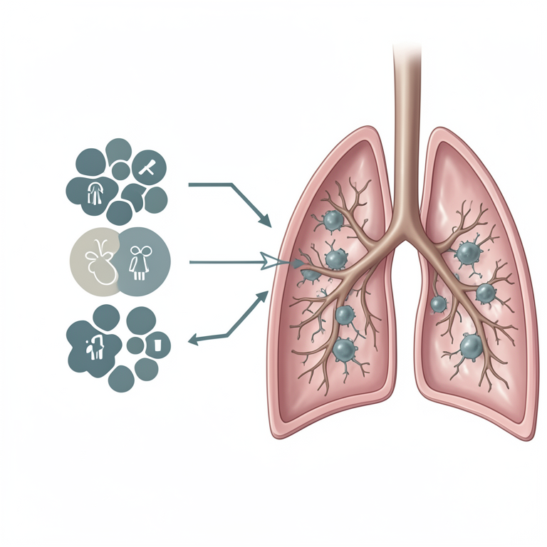
Conceptual Model of TB Causation
AI-generated conceptual illustration (Mycobacterium tuberculosis bacteria and human lung tissue). It explains the idea and does not show study data.
View source evidence ↗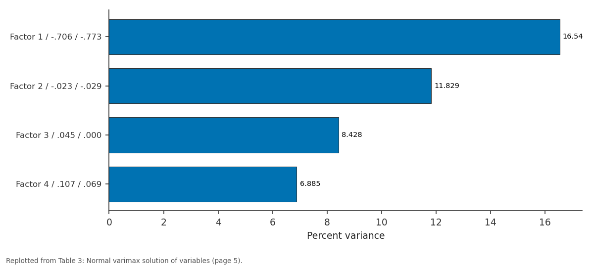
Percent variance: Factor 1 / -.706 / -.773 vs Factor 2 / -.023 / -.029 vs Factor 3 / .045 / .000 vs Factor 4 / .107 / .069
Replotted from Table 3 (page 5) of the original paper. Every bar is the paper's own table value.
View source evidence ↗Figures & tables
From the original paper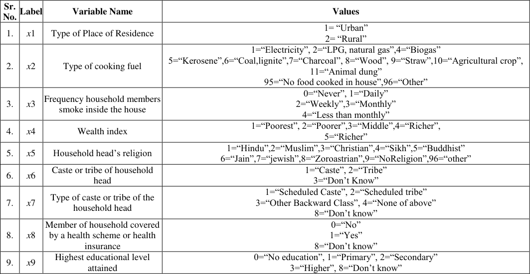 Table 1
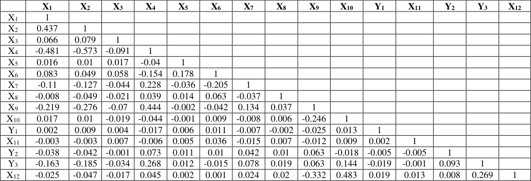 Table 2
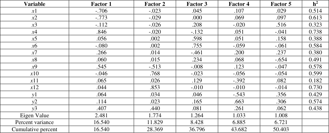 Table 3
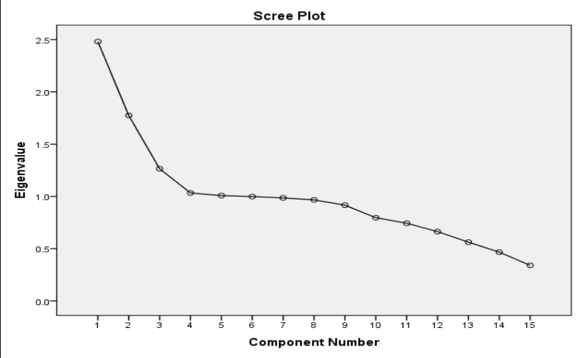 Figure 1
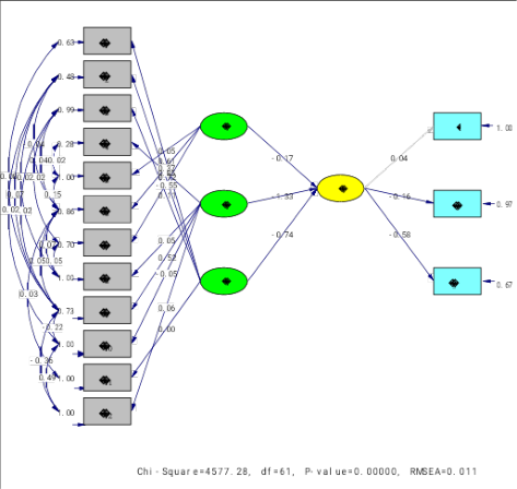 Figure 2
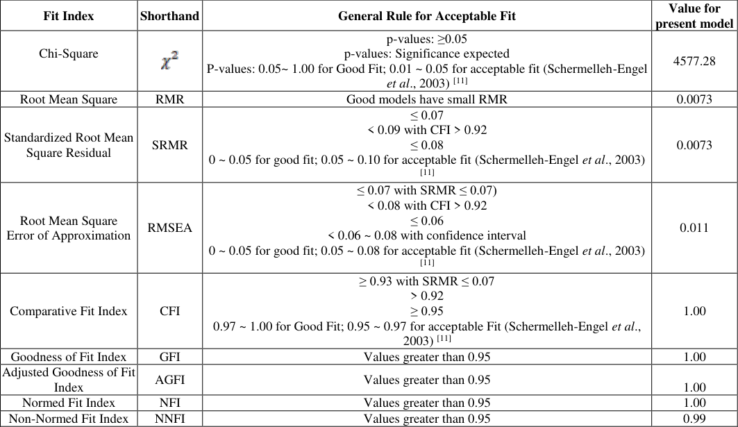 Table 3
 Table 4
Introduction
According to the World Health Organization (WHO), tuberculosis (TB) is a major global public health concern, with an estimated 10.4 million new cases and 1.7 million deaths occurring in 2016 (WHO, 2017) [14] . India is one of the countries with a high burden of TB, accounting for 26% of global cases and 24% of the gap between projected TB incidence and the number of patients newly diagnosed in 2020 (WHO, 2021) [15] . TB is caused by the bacterium Mycobacterium Tuberculosis and is transmitted through the air when an infected person talks, coughs, or sneezes. It is a leading cause of death among HIV patients and is the 9th leading cause of death worldwide (WHO, 2021) [15] . The WHO has designated India as one of 22 high-burden TB countries, along with countries in Africa, Southeast Asia, and the Western Pacific region (WHO, 2021) [15] . In response to this significant public health challenge, the Government of India has set a goal of eliminating TB by 2025. To achieve this goal, it will be necessary to increase access to diagnosis and treatment, improve infection control measures, and implement prevention strategies such as vaccination and the use of preventive therapy. It will also be important to address social and economic factors that contribute to the spread of TB, such as poverty, malnutrition, and poor housing conditions. The surroundings influence health, and the health of the poorest people is most jeopardized by their living conditions. Researchers have attempted to determine the prevalence of TB in various locations of India (ICMR, 1955-1958; Goyal et al., 1978, Kollappan 1992; Katiyar et al., 1994; Malhotra et al., 1996; Radhakrishna 2001; Gopi et al., 2001) [4,3,8,7,9,10,2] . There are many factors that influence and cause TB sickness. Moreover, these factors are highly inter-correlated causing additional complexity. Traditional statistical methodologies are unable to account for the complexity of TB causation. Such complex phenomena can be statistically modelled and tested using Structural Equation Modelling (SEM) by modelling the interactions among independent and dependent variables simultaneously. SEM is a statistical technique that allows researchers to model the interactions among multiple independent and dependent variables simultaneously, taking into account the complexity of the relationships between these variables. This makes it a useful tool for studying the multiple factors that contribute to TB and their interrelationships. The results of these studies demonstrate the usefulness of SEM for understanding the complex relationships between various factors and TB incidence, and for identifying potential interventions to reduce the burden of TB. There have been several research studies that have used structural equation modeling (SEM) to examine the factors that influence the incidence of tuberculosis (TB) in different locations. Wardani et al. (2014) [13] used SEM to examine the effect of social determinants and risk factors on TB incidence in Bandar Lampung municipality, Indonesia. The results of this study showed that social determinants, such as low income, low education level, and overcrowding, were significantly associated with an increased risk of TB. Tola et al. (2017) [12] used SEM to investigate the effect of sociodemographic factors and patients' health beliefs on TB treatment adherence in Ethiopia. The results of this study showed that socio-demographic factors, such as age, education level, and occupation, were significantly associated with TB treatment adherence. Anwar et al. (2018) [1] used SEM to identify the determinants of TB in children in the Banyumas district of Central Java, Indonesia. The results of this study showed that several factors were significantly associated with the risk of TB in children, including low income, low education level, and living in a www.extensionjournal.com household with a TB patient. The aim of carrying out present study using structural equation modeling (SEM) is to identify the latent factors that contribute to the causation of tuberculosis (TB) and other related ailments.
Materials and Methods
The current study aims to identify the latent factors that may contribute to the causation of tuberculosis (TB) and other related ailments using data from the National Family Health Survey (NFHS) 2015-2016. SEM will be utilized in the analysis of the data, which includes various demographic and health-related variables such as place of residence, type of cooking fuel, frequency of household members smoking inside the home, wealth index, religion of the household leader, household head's caste or tribe, health insurance coverage, highest educational level, current marital status, TB diagnosis, smoking habits, anemia levels, Body Mass Index (BMI), and age. After screening for missing data, the final sample size will consist of 6,62,509 observations. It will be assumed that the data follows an asymptotical normal distribution based on the central limit theorem, and the variables of BMI and age will be coded for analysis. The SEM analysis will seek to quantify and test the interrelatedness of these variables with the measured outcomes. Latent variables, or unobserved factors that may influence the occurrence of tuberculosis (TB) and other related ailments, were identified using various statistical techniques. One method used was Exploratory Factor Analysis (EFA), which employed the principle component method to identify the components that may contribute to TB. Significant factor loadings were then used to identify various constructs. In addition, a theoretical model was proposed based on prior knowledge and constructs were identified using measured independent variables. However, both approaches resulted in different constructs, and the structural equation models did not converge to an optimal solution. To address this, the factors obtained from both methodologies were combined, resulting in the development of a convergent measurement and structural equation model that fit well to the data and produced values for various fit indices within the prescribed limits. This final model may be used to better understand the relationships between latent variables and TB causation. Structural Equation Modeling (SEM) consists of two models viz. measurement model and structural model which are discussed in the following sequel.
Measurement Models
The measurement model for endogenous variables or dependent variable y is given by (1) and measurement model for exogenous variable or independent variable x is given by (2) Where, x = (q × 1) vector of exogenous indicator/manifest variables y = (p × 1) vector of endogenous indicator/manifest variables ξ = (n × 1) vector of exogenous latent constructs with mean 0 and variance Φδ η = (m × 1) vector of endogenous latent constructs δ = (q × 1) vector of errors of measurement with mean 0 and variance Θδ ε = (p × 1) vector of errors of measurement with mean 0 and variance Θε Λx= (q × n) matrix of factor loadings Λy= (p × m) matrix of factor loadings
Structural Equation Model
The structural equation model is given by 3. Cov(δ) = E(δδ') = Θδ q x q is var/cov matrix of measurement error associated with observed variables x 4. Cov(ε,δ') = E(ε,δ') = Θδε q x q is var/cov matrix of measurement error associated with observed variables y 5. Cov(ζ) = E(ζζ') = Ψm x m Also, the model implied variance/covariance matrix Σ(θ) is given by
The covariance matrix implied by the model is comprised from three separate correlation matrices, i.e., correlation/ covariance matrix of the observed variable y in terms of
Parameters Estimation and Model Evaluation
In structural equation modeling (SEM), the estimation of model parameters involves determining the values of the parameters that best fit the data. There are several methods that can be used to estimate model parameters in SEM, including maximum likelihood estimation, least squares estimation, and generalized least squares estimation. In present study, maximum likelihood method was used for estimation of model parameters. This method leads to estimates for the parameters θ which maximize the likelihood L that the empirical covariance matrix S is drawn from a population for which the model-implied covariance matrix Σ(θ) is valid. The log-likelihood function log L to be maximized is
Where N is the sample size, θ is the parameter vector, Σ(θ) is the model-implied covariance matrix and c is a constant that contains terms of the Wishart distribution that do not change once the sample is given Maximizing log L is equivalent to minimizing the function
FML is the value of the fitting function evaluated at the final estimates and p is the number of observed variables. In addition to estimating model parameters, it is also important to evaluate the fit of the model to the data. Fit indices are statistical measures that can be used to assess the degree to which the model fits the data. The overall fit of the model is tested by chi-square test statistic, the goodness-of-fit index (GFI), the adjusted goodness-of-fit index(AGFI), the root mean square residual (RMR) (Joreskog and Sorbom, 1989) [6] and model modification index. These criteria are based on differences between the observed (S) matrix and the model implied (∑) variance-covariance matrix. A model with a good fit to the data will have fit indices within the acceptable range, whereas a model with a poor fit will have fit indices outside of this range.
Results and Discussion
In the current study, data from the National Family Health Survey (NFHS) 2015-16 were used. A total of 15 variables were included in the analysis, which may influence the causation of TB and related ailments. The labels and coding for these variables are presented in the Table 1.
Identification of factors responsible for the causation of TB and other ailments
In this study, data from the National Family Health Survey (NFHS) 2015-16 were analyzed to identify latent variables associated with the causation of TB and related ailments. The Exploratory Factor Analysis (EFA) method was initially used to identify these factors. The principal component method of EFA identified five latent variables contributing to TB causation. The correlation between variables is presented in Table 2.
| — | X1 | X2 | X3 | X4 | X5 | X6 | X7 | X8 | X9 | X10 | Y1 | X11 | Y2 | Y3 | X12 |
|---|---|---|---|---|---|---|---|---|---|---|---|---|---|---|---|
| X1 | 1 | ||||||||||||||
| X2 | 0.437 | 1 | |||||||||||||
| X3 | 0.066 | 0.079 | 1 | ||||||||||||
| X4 | -0.481 | -0.573 | -0.091 | 1 | |||||||||||
| X5 | 0.016 | 0.01 | 0.017 | -0.04 | 1 | ||||||||||
| X6 | 0.083 | 0.049 | 0.058 | -0.154 | 0.178 | 1 | |||||||||
| X7 | -0.11 | -0.127 | -0.044 | 0.228 | -0.036 | -0.205 | 1 | ||||||||
| X8 | -0.008 | -0.049 | -0.021 | 0.039 | 0.014 | 0.063 | -0.037 | 1 | |||||||
| X9 | -0.219 | -0.276 | -0.07 | 0.444 | -0.002 | -0.042 | 0.134 | 0.037 | 1 | ||||||
| X10 | 0.017 | 0.01 | -0.019 | -0.044 | -0.001 | 0.009 | -0.008 | 0.006 | -0.246 | 1 | |||||
| Y1 | 0.002 | 0.009 | 0.004 | -0.017 | 0.006 | 0.011 | -0.007 | -0.002 | -0.025 | 0.013 | 1 | ||||
| X11 | -0.003 | -0.003 | 0.007 | -0.006 | 0.005 | 0.036 | -0.015 | 0.007 | -0.012 | 0.009 | 0.002 | 1 | |||
| Y2 | -0.038 | -0.042 | -0.001 | 0.073 | 0.011 | 0.01 | 0.042 | 0.01 | 0.063 | -0.018 | -0.005 | -0.005 | 1 | ||
| Y3 | -0.163 | -0.185 | -0.034 | 0.268 | 0.012 | -0.015 | 0.078 | 0.019 | 0.063 | 0.144 | -0.019 | -0.001 | 0.093 | 1 | |
| X12 | -0.025 | -0.047 | -0.017 | 0.045 | 0.002 | 0.001 | 0.024 | 0.02 | -0.332 | 0.483 | 0.019 | 0.013 | 0.008 | 0.269 | 1 |
Table text extracted from the original PDF; superscript letters are shown inline. The original table image is below.
View original table image
Table 1: Codes and description of variables
Table 1: Codes and description of variables
Sr.
Sr.
Label Variable Name Values
Label Variable Name Values
x1
Type of Place of Residence 1= "Urban" 2= "Rural"
x2
Type of cooking fuel 1="Electricity", 2="LPG, natural gas",4="Biogas" 5="Kerosene",6="Coal,lignite",7="Charcoal", 8="Wood", 9="Straw",10="Agricultural crop", 11="Animal dung" 95="No food cooked in house",96="Other"
x3
Frequency household members smoke inside the house 0="Never", 1="Daily" 2="Weekly",3="Monthly" 4="Less than monthly"
x4
Wealth index 1="Poorest", 2="Poorer",3="Middle",4="Richer", 5="Richer"
x5
Household head's religion 1="Hindu",2="Muslim",3="Christian",4="Sikh",5="Buddhist" 6="Jain",7="jewish",8="Zoroastrian",9="NoReligion",96="other"
x6
Caste or tribe of household head 1="Caste", 2="Tribe" 3="Don't Know"
x7
Type of caste or tribe of the household head 1="Scheduled Caste", 2="Scheduled tribe" 3="Other Backward Class", 4="None of above" 8="Don't know"
x8
Member of household covered by a health scheme or health insurance 0="No" 1="Yes" 8="Don't know"
x9
Highest educational level attained 0="No education", 1="Primary", 2="Secondary" 3="Higher", 8="Don't know" www.extensionjournal.com
x10
Current marital status 0="Nevermarried",1="Married",2="Livingtogether",3="Widowed",4="Divorced", 5="Not living together", 8="Don't know"
x11
Smoking (Cigarettes in last 24 hours)
0="Doesn't smoke" 94="Smokes pipes, cigars, etc" 12. x12 Age 1="10-20",2="20-30",3="30-40",4="40-50" 13. y1
Suffers from TB 0="No",1="Yes" 14. y2 Anemia Level 1="Severe", 2="Moderate", 3="Mild",4="Not anemic"
15. y3 Body Mass Index 1="1000-2000", 2="2000-3000",3="3000-4000" 4="4000-5000",5="5000-6000"
A rule of thumb for determining the significance of a correlation coefficient is based on the relationship between the sample size and the correlation. If , correlation is considered significant, otherwise it is not. For the current sample, a value of greater than 0.0025 is considered significant. Correlation coefficients between variables in bold in the table are significant. The number of factors to be retained was determined by examining the scree plot (Figure 1) and using the Kaiser criterion (eigenvalue greater than 1). Both criteria indicated that five components should be retained. Additionally, the Kaiser-Meyer-Olkin measure of sampling adequacy (0.689) also suggested that a five-factor solution was appropriate. The measure of communality (h 2 ) represents the proportion of the variance of a variable that is common to other variables in the set and reflects the percentage of variation for each of the variables explained by all factors. An examination of the communality values shows that 8 out of the 15 variables had communalities greater than 50%. The normal varimax rotated factor solution was used in the analysis (Table 3), which involves rotating the observed variables to maximize the variance of each variable's loading on a single factor. The rotation continues until convergence is reached, which occurred after 7 iterations in this case. In an ideal scenario, each observed variable would only have a loading of 1 on a single factor, with no loadings on any other factors. However, it is common for observed variables to have significant loadings on multiple factors in practice. In this study, loadings greater than 0.40 were considered significant, while loadings greater than 0.50 were considered highly significant. This is a commonly used threshold for determining the importance of a loading in factor analysis. The analysis identified five latent variables, which were labeled "economic factors", "demographic factors", "social factors", "illness", and "awareness about TB". These latent variables were identified based on factor loadings of the observed variables on them. The "economic factors" latent variable was identified by significant negative loadings on the variables "type of place of residence" (-0.651) and "type of cooking fuel" (-0.514) and a positive loading on the variable "wealth index" (0.739). The "demographic factors" latent variable was identified by significant positive loadings on the variables "current marital status" (0.532), "age" (0.671), and "body mass index" (0.466), as well as a negative loading on the variable "highest education level attained" (-0.515). The "social factors" latent variable was identified by significant positive loadings on the variables "Household head's religion" (0.517) and "caste or tribe of household head" (0.501), as well as a negative loading on the variable "type of caste or tribe of household head" (-0.432). The "illness" latent variable was identified by a significant positive loading on the variable "anemia level" (0.625) and a negative loading on the variable "suffers from TB" (-0.504). The "awareness about TB" latent variable was identified by negative (-0.441) and positive (0.491) loadings on the variables "member of household covered by a health scheme or health insurance" and "frequency of household member smoke inside house", respectively. The total variance explained by these five latent variables was 50.403%. When the sample size is small, fewer principal components may be required to explain the same amount of variance in the data. This is because the leading eigenvalues, which correspond to the largest variances in the data, tend to be overestimated when the sample size is small, while the trailing eigenvalues, which correspond to the smaller variances, are underestimated. Conversely, if the sample size is large, it is more likely that a greater number of principal components will be needed to explain the same amount of variance in the data, as the leading eigenvalues are less likely to be overestimated and the trailing eigenvalues are less likely to be underestimated (Jollife, 2002, Section 3.6) [5] . In the current study, it was found that the first five principal components were able to explain a substantial amount of the variance in the data (50.403%). Additionally, the variables for smoking, body mass index, and highest education level displayed significant loadings on the first two components, indicating complex relationships. Although it is theoretically unlikely that these latent variables would be uncorrelated in the population, the factor analysis served as a starting point for further investigation using structural equation modeling with latent variables. This additional analysis can help to statistically test and clarify the somewhat ambiguous findings from the initial factor analysis. www.extensionjournal.com Health factors are measured by variables such as health insurance coverage, smoking status, anemia level, body mass index, and presence of TB. Demographic factors are represented by age and current marital status. This approach to grouping variables into latent constructs allows for a deeper understanding of the relationships between these variables and how they may be related to one another.
| Variable | Factor 1 | Factor 2 | Factor 3 | Factor 4 | Factor 5 | h2 |
|---|---|---|---|---|---|---|
| x1 | -.706 | -.023 | .045 | .107 | .029 | 0.514 |
| x2 | -.773 | -.029 | .000 | .069 | .097 | 0.613 |
| x3 | -.112 | -.026 | .208 | -.020 | .516 | 0.323 |
| x4 | .846 | -.020 | -.132 | .051 | -.041 | 0.738 |
| x5 | .056 | .002 | .598 | .051 | .158 | 0.388 |
| x6 | -.080 | .002 | .755 | -.059 | -.061 | 0.584 |
| x7 | .266 | .014 | -.461 | .200 | .237 | 0.380 |
| x8 | .060 | .015 | .234 | .068 | -.654 | 0.491 |
| x9 | .545 | -.513 | -.008 | .123 | -.047 | 0.578 |
| x10 | -.046 | .768 | -.023 | -.056 | -.054 | 0.599 |
| x11 | .065 | .026 | .129 | -.392 | .082 | 0.182 |
| x12 | .044 | .853 | -.010 | -.010 | -.014 | 0.730 |
| y1 | .064 | .034 | .046 | -.543 | .356 | 0.429 |
| y2 | .114 | .023 | .165 | .663 | .306 | 0.574 |
| y3 | .407 | .440 | .081 | .261 | .062 | 0.438 |
| Eigen Value | 2.481 | 1.774 | 1.264 | 1.033 | 1.008 | |
| Percent variance | 16.540 | 11.829 | 8.428 | 6.885 | 6.721 | |
| Cumulative percent | 16.540 | 28.369 | 36.796 | 43.682 | 50.403 |
Table text extracted from the original PDF; superscript letters are shown inline. The original table image is below.
View original table image
Structural equation model
In the current study, exploratory factor analysis was used to identify five latent variables that could be included in a structural equation model. Initially, a model was proposed using these latent variables, but it did not converge to an optimal solution after 50 iterations. Therefore, the model was revised using both theoretical knowledge and some of the constructs identified by the exploratory factor analysis. Some variables were found to be heavily loaded on two factors, while the indicator variable for smoking was not significantly loaded on any variables in the initial model. This model had poor fit statistics, so modifications were made to the residual matrices and indicator variables were added or removed from the latent constructs based on the largest modification indices. After each change, the model parameters were re-estimated and tested. Eventually, the model converged to an optimal solution with acceptable fit statistics, and the final model is depicted in a path diagram (Figure 2). The endogenous measurement model was obtained as (7) And the exogenous measurement model is given by ( 8)
The final structural equation is given by ( 9)
Where the latent error terms have the following covariance matrix with only one element
The final structural equation model in the present study is depicted in a path diagram (Figure 2), which shows that there are three exogenous latent variables (ξ1, ξ2, ξ3) and one endogenous latent variable (η1). These latent variables are measured by a combination of observed variables. The exogenous latent variable ξ1 is measured by household Initially, a restricted model was fitted in which the offdiagonal elements of the variance-covariance matrix were set to zero. Although this model converged, the fit statistics (such as the chi-square statistic and Root Mean Square Error Approximation) were not within the acceptable range. In order to improve the fit of the model, the restrictions on the independence of the error terms were removed in the measurement model. Based on the largest modification indices, some of the error terms in the measurement model were allowed to correlate. This resulted in a significant decrease in the fit statistics (such as the chi-square statistic and RMSEA) and brought them within the acceptable range. This fine-tuning process can help to improve the overall fit of the model and make it more representative of the data. www.extensionjournal.com Schermelleh-Engel et al. (2003) [11] suggested that the value of chi-square depends upon the sample size i.e., as the sample size increases, the value of this statistic increases and model might be rejected even though the discrepancy between the model-implied covariance matrix is irrelevant. In present study, the size of the sample was 6, 62,509 therefore large value of chi-square statistic cannot pose a big problem for significance testing. The initial model was improved by allowing for the measurement errors of certain exogenous variables (e.g., X1 and X9, X2 and X6, X2 and X8) to correlate and by including indicator variables that were significantly loaded on latent variables, as suggested by the largest modification indices. On removing the restriction on several off-diagonal elements of , and as given in equation ( 10), ( 11) and ( 12) respectively produced a chisquare value as 4577.28,d.f.=61. No significant correlations were found between the measurement errors of the endogenous variables. The final SEM model also included significant correlations between certain exogenous and endogenous variables (e.g., X6 and Y2, X7 and Y2, X6 and Y3, X9 and Y3, X10 and Y3, and X12 and Y3). The fit indices for the final model were within the prescribed limits, indicating that the model fit the data well. The maximum likelihood estimates of the model parameters, along with tvalues, are presented in Table 4. The perusal of estimates in table 4 indicated that all parameters are significant as they have large t-value.
| Parameter | Estimate | t-value | Parameter | Estimate | t-value |
|---|---|---|---|---|---|
| 0.61 | 470.13 | 1.00 | 575.54 | ||
| 0.72 | 550.77 | 1.00 | 575.09 | ||
| 0.11 | 79.82 | 0.08 | 39.10 | ||
| 0.85 | 315.13 | -0.04 | -40.06 |
Table text extracted from the original PDF; superscript letters are shown inline. The original table image is below.
View original table image
( [11] 4577.28 2003) [11] 1.00
References
12 in the original paper- Anwar MC, Gunawan, Asep Tata, Widyanto T, Suparmin, Marsum, Rajiani I. A structural equation model of tuberculosis (TB) infection in children. Indian J Public Health Res. Dev. 2018;9(8):73-77.
- Gopi PG, Subramani R, Radhakrishna S, Kolappan C, Sadacharam K, Devi TS, et al. A baseline survey of the prevalence of tuberculosis in a community in the South India at the commencement of a DOTS programme. Int. J Tuberc. Lung Dis. 2003;7(12):1154-62.
- Goyal SS, Mathur GP. Tuberculosis trends in urban community. Indian J Tuberc. 1978;25(2):77-82.
- Katiyar SK, Singh RP, Chaudhri S, Singh KP, Chandershekhar, Srivastava AK. Prevalence of tuberculosis in BCG vaccinated and unvaccinated and among tuberculin reactors and non-reactors in rural population as detected by a mobile chest clinic. Indian J Tuberc. 1994;41(3):183.
- Kolappan C. Prevalence of tuberculosis in North Arcot district of Tamil Nadu. Indian J Tuberc. 1992;39(2):134.
- Malhotra P, Abrol Kaur V, Dhar S, Singh A, Kaul S, Raina RK. Prevalence of tuberculosis in Kishtwar Tehsil of Jammu region in Jammu and Kashmir State. J 350 www.extensionjournal.com Indian Med Assoc. 1996;94(9):334-337.
- Radhakrishna S. Trends in the prevalence and incidence of tuberculosios in south India. Int J Tuberc Lung Dis. 2001;5(2):142-157.
- Engel SK, Moosbrugger H, Miller H. Evaluating the fit of structural equation models: Tests of significance and descriptive goodness-of-fit measures. Methods Psychol Res Online. 2003;8:23-74.
- Tola HH, Karimi M, Yekaninejad MS. Effects of sociodemographic characteristics and patients health beliefs on tuberculosis treatment adherence in Ethiopia: a structural equation modelling approach. Infect Dis Poverty. 2017;6:167.
- Wardani DWSR, Lazuardi L, Mahendradhata Y, Kusnanto H. Structured equation model of tuberculosis incidence based on its social determinants and risk factors in Bandar Lampung, Indonesia. Open J Epidemiol. 2014;4:76-83.
- World Health Organization. Global tuberculosis report 2017. Geneva: World Health Organization; c2017.
- World Health Organization. Global tuberculosis report 2021. Geneva: World Health Organization; c2021.