
Research article · 2024 · Full text
International Journal of Statistics and Applied MathematicsParticle swarm optimization algorithm-based nonlinear LS-SVM model for modelling and forecasting time-series data
Volume 9(2) · Pages 10–16 · DOI: 10.22271/maths.2024.v9.i2a.1638 ↗
Research areasAdvanced Algorithms and ApplicationsNeural Networks and ApplicationsTime Series Analysis and Forecasting
Abstract
Author-writtenIn this article, a novel Nonparametric, Nonlinear Least Squares Support Vector Machine (LS-SVM) methodology is thoroughly studied. The Particle Swarm Optimization (PSO), which is a very efficient population-based global stochastic optimization technique, is employed to estimate the hyper-parameters and time lag of Nonlinear LS-SVM model for time-series modelling. Relevant computer program is written in MATLAB function (m file). The MATLAB and STATISTICA software packages are used for carrying out data analysis. Subsequently, as an illustration, the methodology was applied to all-India annual rainfall time-series data. Superiority of this approach over ANN model is demonstrated using Root Mean Square Error (RMSE) and Mean Absolute Percent Error (MAPE) criteria for data under consideration.
Summary
Source-checkedPlain-language reading of the full paper, prepared with AI and checked against the text. Each point links to the authors' own words.
Why it matters
- Traditional time-series analysis often relies on ARIMA models, but these are limited because they are linear. View evidence ↗
- Nonlinear Least Squares Support Vector Machines (LS-SVM) offer faster convergence and higher accuracy than standard SVR by using a linear least squares criterion. View evidence ↗
The question
- The study aims to investigate the Nonlinear LS-SVM methodology and use Particle Swarm Optimization (PSO) to determine the best hyper-parameters and time lags. View evidence ↗
What they did
- The researchers used all-India annual rainfall data (in mm) from 1871 to 2011 as an illustrative dataset. View evidence ↗
- The dataset was split into a training set (1871–1999) and a testing set (2000–2011). View evidence ↗
- The PSO algorithm was configured with 100 particles, 500 maximum iterations, acceleration factors c1=c2=2.05, and an inertia weight decreasing linearly from 0.9 to 0.1. View evidence ↗
- The benchmark ANN model consisted of a three-layer feed-forward network using a sigmoid activation function. View evidence ↗
What they found
- The PSO+LS-SVM model achieved a lower Cross-Validation Mean Square Error (CV-MSE) of 0.029 compared to 0.031 for the standard LS-SVM model. View evidence ↗
- For the testing dataset, the PSO+LS-SVM model remained the most accurate with an RMSE of 73.957 and MAPE of 6.609, compared to LS-SVM (RMSE 77.420) and ANN (RMSE 80.791). View evidence ↗
What it means
- The authors conclude that the PSO+Nonlinear LS-SVM model is superior to both the Grid search-based LS-SVM and the ANN model in terms of accuracy for rainfall forecasting. View evidence ↗
Visual summary
2 visualsIllustrations explain the paper; charts are replotted from the paper's own table values.

PSO Optimization Process
AI-generated conceptual illustration (A 3D mathematical landscape representing a cost function surface). It explains the idea and does not show study data.
View source evidence ↗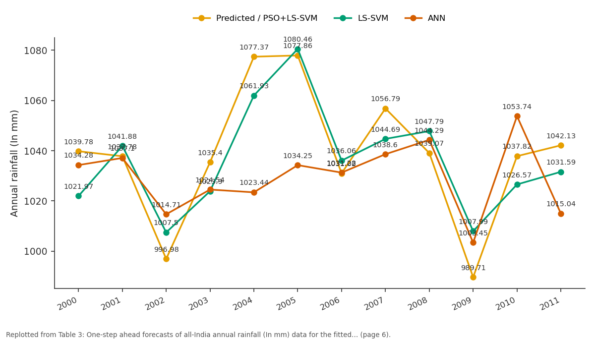
Predicted / PSO+LS-SVM and LS-SVM and more: 2000 vs 2001 vs 2002 vs 2003 vs 2004
Replotted from Table 3 (page 6) of the original paper. Every bar is the paper's own table value.
View source evidence ↗Figures & tables
From the original paper Table 1
 Table 2
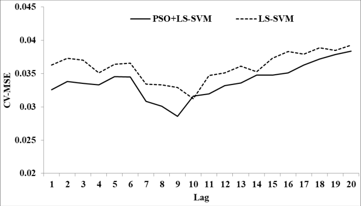 Figure 1
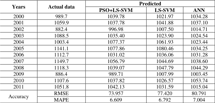 Table 3
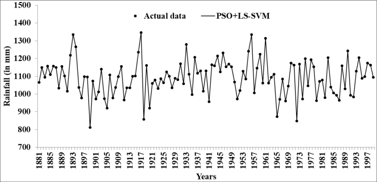 Figure 2
Introduction
Analysis of time-series data has usually been carried out by employing the well-known Box-Jenkins Autoregressive Integrated Moving Average (ARIMA) family of models. However, the main disadvantage of these approaches is that the underlying models are 'linear'. During the last three decades or so, the area of "Nonlinear time-series modelling" has rapidly been growing. Here, there are basically two approaches, viz. Parametric or Nonparametric. However, quite often it is noticed that there is no appropriate parametric form to describe the time-series data under consideration in a satisfactory manner. In such cases, 'Nonparametric regression methodology' may be employed (Chandran and Prajneshu, 2007) [1] . During the last few years, another nonparametric methodology of 'Wavelet analysis' has emerged. The novel idea of wavelets is that these are localized in both time and space, whereas traditional Fourier bases are localized only in frequency but not in time. Wavelet analysis can be carried out either in the Time domain or in the Frequency domain. Ghosh et al. (2010) [2] investigated the wavelet approach in the frequency domain for analyzing time-series data. Chattopadhyay and Chattopadhyay, 2013 [3] was reported that in the last decade, with the success of the backpropagation algorithm for computing derivatives, the Artificial Neural Networks (ANN) methodology has been extensively used. However, the main drawbacks of this methodology are that the resultant models generally over fit the data and that the solution gets trapped in local minima. The methodology, which does not suffer from the above limitations, is the Support Vector Machine/Regression (SVM / SVR) methodology developed by Vapnik (2000) [4] . This Nonparametric methodology is very promising for nonlinear regression analysis. It implements the Structural Risk Minimization principle, which has been shown to be superior to the traditional Empirical Risk Minimization principle implemented in ANN models. An excellent description of various aspects of SVR methodology is given in Smola and Scholkopf (2004) [5] . Later on, the Least Squares version of SVM, known as the Least Squares-Support Vector Machine (LS-SVM) was proposed by Suykens et al., 2002 [6] for nonlinear regression analysis.
A heartening aspect of Nonparametric Nonlinear LS-SVM as compared to standard Nonlinear SVR for regression problems is that it applies linear least squares criterion to the loss function with only equality type constraints to obtain a set of linear equations instead of epsilon insensitive loss function with inequality type constraints to form traditional convex Quadratic Programming problem. This leads to the advantages of fast convergence, high accuracy and low computational efforts. Despite the superior features of the above methodology, its generalization and efficiency are sensitive to the values of hyperparameters as well as the dimension of the input vector (the lagged observations). Therefore, the selection of optimal hyperparameters and time lags is an important step in Nonlinear LS-SVM modelling. To this end, Chen and Wang (2007) [7] discussed the advantages and disadvantages of various efficient estimation procedures and also proposed real-valued Genetic algorithm (GA) technique. However, its main drawback is that the GA-SVR approaches cannot optimize all Nonlinear SVR's hyperparameters and time lags simultaneously. Moreover, GAs are capable of finding the solution through evolution operators, such as crossover and mutation. Evolution is inductive. In reality, life does not always evolve towards a good solution. Fortunately, a very efficient population-based stochastic optimization algorithm, viz. The Particle Swarm Optimization (PSO) technique is capable of rectifying the above limitations (Parsopoulos and Vrahatis, 2010) [8] . In contrast to GA, which exploits the competitive characteristics of biological evolution, PSO simulates cooperative and social behaviour, such as fish schooling, birds flocking, or insects swarming. In this article, our purpose is to thoroughly study the Nonlinear LS-SVM methodology and PSO-based estimation procedure to estimate its optimal hyper-parameters as well as time lags. The relevant computer program is written in MATLAB function (m file). Finally, as an illustration, all-India annual rainfall time-series data are considered. The superiority of the developed model is demonstrated over the ANN approach.
Description of the methodologies 2.1 Nonlinear Least Squares Support Vector Machine (LS-SVM)
Suppose the training data set is
is the i th input data, R y i is the i th target data and N corresponds to the size of the training data. In the primal weight space, the Nonlinear LS-SVM function for regression is given by.
(.) is a nonlinear function, which maps the input space into a higher dimensional feature space, h n R w is the weight vector and b is the bias term. The Nonlinear LS-SVM for regression formulation can be described as.
is the weight vector in primal weight space, R e i are error variables and b is the bias term. Note that the cost function J P consists of a sum of squared fitting error and regularization term in primal feature space. The relative importance of these two terms is determined by the positive real constant γ. In the case of noisy data, one avoids over-fitting by taking a smaller γ value. The weight vector w can be infinite-dimensional, which makes a calculation of w as impossible, in general. The Lagrangian function can be constructed as.
Where α i , i=1, 2,…,N are Lagrangian multipliers, also called support values. The Karusha-Kuhn-Tucker (KKT) conditions for optimality are given by partially differentiating L.
After eliminating 'w' and 'e i ', optimization problem can be transferred into the following linear solution system in dual space: , 0 1 1
In the above, K(x i , x j ) is called the inner-product kernel function. Thus, Nonlinear LS-SVM for regression is obtained as
Where i and b are solutions of the linear system.
For a univariate time-series forecasting problem, the dimension of input vectors is the past lagged observations. The Nonlinear LS-SVM model performs a nonlinear functional mapping from the past observations to the future value as:
Where y t is the output value, p is the dimension of the input vector and t is the error term.
Several kernel functions K(x i ,x j ) are available in the literature, like the Polynomial function, Gaussian kernel, and Radial-basis function (RBF). In this article, the RBF kernel function
is used to train the Nonlinear LS-SVM model, since it has only one hyper-parameter that needs to be pre-determined and yields good performance for nonlinear time-series forecasting. Training Nonlinear LS-SVM with RBF kernel function is required to be optimized through two hyperparameters, viz. Regularization parameter gamma (γ) and Kernel bandwidth parameter sigma (), which may affect Nonlinear LS-SVM generalization performance. Also, the important task of Nonlinear LS-SVM modelling is to estimate the optimal dimension of input vector p (i.e. the lagged observations). However, in practice, the choice of p is difficult; often trial and error method is conducted. To this end, PSO is employed to optimize Nonlinear LS-SVM hyper-parameters as well as time lag p simultaneously.
Development of Particle Swarm Optimization Algorithm (PSO) for Nonlinear LS-SVM
The PSO is a population-based stochastic optimization search method, i.e. it exploits a population of potential solutions to probe the search space concurrently, proposed by Kennedy and Eberhart in 1995 (Parsopoulos and Vrahatis, 2010 [8] ). The population is called the 'swarm' and its individuals are called the 'particles' Let
, i=1, 2,…, N. Indices are arbitrarily assigned to particles, while N is a user-defined parameter of the algorithm. The PSO algorithm investigates solution space using a set of particle vectors that are updated from iteration to iteration. Each particle is a potential solution, characterized by three quantities: Its velocity , ) ,..., , (
and personal best position . ) ,..., , (
Let t denote the current iteration and gbest denote its global best position achieved so far by any of its particles. Initially, the swarm is randomly dispersed within the search space, and random velocity is assigned to each particle. Particles interact with one another by sharing information to discover the optimal solution. Each particle moves in the direction of its personal best position (pbest) and its global best position (gbest). To search optimal solution, each particle changes its velocity according to the cognitive and social parts as given by eq. ( 10) and move to a new potential solution by updating its position based on the eq. (11).
Where V ij , X ij and pbest ij are respectively velocity, position and pbest position of particle i on the j th dimension and gbest j is the j th dimension gbest position among all particles at iteration t. The R 1 and R 2 are random values, which are mutually independent and uniformly distributed over [0,1] , is constraint factor used to control the velocity weight, whose value is usually set equal to 1.
Positive constants c 1 and c 2 are usually called the "acceleration factors". Factor c 1 is sometimes referred to as a "cognitive" parameter, while c 2 is referred to as a "social" parameter. The w(t) is the inertia weight at iteration t and is used to balance global exploration and local exploitation. This can be determined by. , )
Where t is current iteration number, w up and w low are desirable lower and upper limits of w, and T max is the maximum number of iterations. The process of optimizing the Nonlinear LS-SVM model hyper-parameters as well as time lags by PSO is described in the following steps.
Data preparation:
The time-series data points are divided into two parts: (i) Training dataset, which is used only for building the model, and (ii) Testing dataset, which is used for validation of the model.
Initialization and PSO parameter setting:
First, set the time lag one to the maximum number of lags to be considered as the dimension of the input vector to estimate optimal time lag p. Then, Nonlinear LS-SVM model hyper-parameters γ and σ (Here n=2) are directly coded with real values within a given search space to randomly generate N number of initial particles of swarm set S. The search space of hyper-parameters γ and are respectively limited to ranges of [γ min , γ max ] and [σ min , σ max ].
Also randomly generate initial particle velocity (V i ) limited to the range [-V max ,V max ]. 3. Evaluate each particle's fitness: For each candidate particle of initial particles, train the Nonlinear LS-SVM model using kfold cross-validation to evaluate the minimum value of fitness function, defined as the cross-validation Mean Square Error (CV-MSE):
Where y j and j y ˆare respectively actual and predicted values of the validation subset, m is the number of samples in the validation subset and k is the number of folds for cross-validation. Then, update the personal best position pbest i of each particle and the global best position gbest achieved so far by any of its particles according to minimum fitness value. 1. Now set the iteration number (t) one to the maximum number of iterations and evaluate inertia weight w(t) at iteration t using eq. (12). 2. Compute and update the velocity of each particle using eq. (10). 3. Compute and update the position of each particle using eq. (11). 4. Termination: Repeat the search process from Step (iii) to Step (vi) until stop conditions, such as maximum iteration, are met.
Finally, optimal hyper-parameters and time lag p are utilized to build the Nonlinear LS-SVM model on the training dataset and the testing dataset is used to validate the fitted model. To perform the above tasks, the LS-SVMLab, Version 1.8 toolbox, developed by De Brabanter et al. (2011) [9] for the MATLAB 2012a software platform, is employed for training the Nonlinear LS-SVM model. We have written MATLAB function (m file) code for estimating hyper-parameters of the Nonlinear LS-SVM model using the PSO algorithm, and the same is appended as ANNEXURE-1.
An illustration
As an illustration, all-India annual rainfall (in mm) time-series data for the period 1871 to 2011, obtained from the website (www.tropmet.res.in) of the Indian Institute of Tropical Meteorology, Pune, India are considered. The data points for the period 1871 to 1999 are used as a training dataset and the remaining data points for the period 2000 to 2011 are used as a testing dataset. Note that, before training the model, training and testing data points are normalized to the range [0, 1] separately using eq. ( 14), which can improve the generalization power of Nonlinear LS-SVM. Through the initial experiment, the parameters of the PSO technique were set as follows: 100 initial particles (so that it is enough to cover the search space within the limited iterations based on experimental runs), 500 maximum iterations, inertia weight is initially set as 0.9 and reduced to 0.1 linearly according to eq. ( 16) and c 1 =c 2 =2.05. The searching range of Nonlinear LS-SVM model hyper-parameters γ and were respectively set in the range [0.001,1000] and [0.001,100] and their velocity bounds were respectively set to be in the range [-499. 99, 499. 99] and [-49.99, 49.99]. For comparison purposes, Grid search, the most commonly used method for estimating optimal hyper-parameters was also employed. In the training stage, the PSO and Grid search techniques were employed to estimate optimal hyper-parameters and time lag of Nonlinear LS-SVM based on 10-fold cross-validation and the results along with CV-MSE values are reported in Table 1. The following Fig. 1 illustrates the CV-MSE estimates over a different lag period by Grid Search and PSO techniques. separately using eq. ( 14). In this article, a typical three-layer feed-forward network with one input layer, one hidden layer and one output layer is used to develop the model. The most commonly used sigmoid activation function for time-series modelling was applied to the input layer to the hidden layer and the hidden layer to the output layer. In the training and testing of the ANN network, the same input lag structure of PSO + Nonlinear LS-SVM model was considered. The network was trained using the Back-Propagation algorithm with a learning rate of 0.001 and the trial and error method was performed to optimize the optimal number of neurons in the hidden layer, which was found to be 9 neurons. Further, Nonlinear LS-SVM models and ANN model are compared based on Root Mean Square Error (RMSE) and Mean Absolute Percent Error (MAPE) respectively given in eq. ( 15) and eq. ( 16). Where, y j is the actual value and j y ˆ is the predicted value, n is the number of samples in the data subset. The RMSE and MAPE for the above-fitted models are computed on the training dataset, which are reported in Table 2.
| Accuracy\Models | PSO+LS-SVM | LS-SVM | ANN |
|---|---|---|---|
| RMSE | 0.125 | 0.1930 | 95.234 |
| MAPE | 0.009 | 0.014 | 7.028 |
Table text extracted from the original PDF; superscript letters are shown inline. The original table image is below.
View original table image
| Model | | | lag | CV-MSE |
|---|---|---|---|---|
| LS-SVM | 593.751 | 0.055 | 10 | 0.031 |
| PSO+LS-SVM | 996.999 | 0.053 | 9 | 0.029 |
Table text extracted from the original PDF; superscript letters are shown inline. The original table image is below.
View original table image
Figures and tables from the paper
| Years | Actual data | Predicted | — | — |
|---|---|---|---|---|
| PSO+LS-SVM | LS-SVM | ANN | ||
| 2000 | 989.7 | 1039.78 | 1021.97 | 1034.28 |
| 2001 | 1059.9 | 1037.78 | 1041.88 | 1037.10 |
| 2002 | 882.4 | 996.98 | 1007.50 | 1014.71 |
| 2003 | 1088.5 | 1035.40 | 1023.90 | 1024.54 |
| 2004 | 1003.4 | 1077.37 | 1061.93 | 1023.44 |
| 2005 | 1141.1 | 1077.86 | 1080.46 | 1034.25 |
| 2006 | 1112.7 | 1031.02 | 1036.06 | 1031.28 |
| 2007 | 1149.7 | 1056.79 | 1044.69 | 1038.60 |
| 2008 | 1118.3 | 1039.07 | 1047.79 | 1044.29 |
| 2009 | 886.4 | 989.71 | 1007.99 | 1003.45 |
| 2010 | 1107.6 | 1037.82 | 1026.57 | 1053.74 |
| 2011 | 1051.8 | 1042.13 | 1031.59 | 1015.04 |
| Accuracy | RMSE | 73.957 | 77.420 | 80.791 |
| MAPE | 6.609 | 6.792 | 7.004 |
Table text extracted from the original PDF; superscript letters are shown inline. The original table image is below.
View original table image
References
5 in the original paper- Chandran KP, Prajneshu. Nonparametric regression approach for modelling and forecasting country's meteorological subdivisions rainfall data. J. Agrometeorol. 2007;8(2):254-259.
- Ghosh H, Paul RK, Prajneshu. Wavelet frequency domain approach for statistical modeling of Indian monsoon rainfall timeseries data. J Statist. Theo. Prac. 2010;4(4):813-825.
- Chattopadhyay S, Chattopadhyay G. A supervised Neural Network model for predicting average summer monsoon rainfall in India. J Ind. Soc. Ag. Statist. 2013;67(1):43-49.
- Smola AJ, Scholkopf B. A tutorial on support vector regression, Statist. Comput. 2004;14:199-222.
- Chen KY, Wang CH. Support vector regression with genetic algorithm in forecasting tourism demand. Tour. Mgmt. 2007;28(1):215-226.