
Research article · 2023 · Full text
International Journal of Statistics and Applied MathematicsBayesian approach to control charts for process precision
Volume 8(6) · Pages 30–40 · DOI: 10.22271/maths.2023.v8.i6a.1400 ↗
Research areasAdvanced Statistical Process MonitoringFault Detection and Control SystemsAdvanced Control Systems Optimization
Abstract
Author-writtenMonitoring process variation is essential to maintain quality of certain product in manufacturing industry. Coefficient of variance (CV) is a relative measure of process variation and inverse coefficient of variance (ICV) measures relative precision. In this paper, control charts for ICV under normal model using Bayesian approach is proposed. The control charts are constructed under noninformative and gamma priors. Their performance is investigated. The proposed control charts are illustrated through examples.
Summary
Source-checkedPlain-language reading of the full paper, prepared with AI and checked against the text. Each point links to the authors' own words.
Why it matters
- Monitoring process variation is critical for maintaining product quality within the manufacturing industry. View evidence ↗
- The inverse coefficient of variance (ICV) is used as a measure of process precision. View evidence ↗
- ICV control charts are useful for quality maintenance in industries producing items like surgical instruments, footwear, apparel, and jewelry. View evidence ↗
The question
- The study aims to develop Bayesian control charts for the inverse coefficient of variance (ICV) under a normal model using noninformative (NI) and gamma priors. View evidence ↗
What they did
- The researchers derived the expected value and variance for both standard ICV and range-based ICV to construct the control charts. View evidence ↗
- The performance of the proposed control charts was evaluated based on power and average run length (ARL). View evidence ↗
- The analysis tested sample sizes of n=15, 20, and 25 to determine the power and ARL of the T control chart under a noninformative prior. View evidence ↗
What they found
- For a fixed sample size, the power of the control chart increases as the shift in the mean (𝑥′) increases and decreases as the shift in ICV (𝜏̂′) increases. View evidence ↗
- For a specific shift in ICV, the power of the control chart increases as the sample size (n) increases. View evidence ↗
- Under both noninformative and gamma priors, increasing the sample size (n) leads to increased power and decreased average run length (ARL) for the T control chart. View evidence ↗
- The range-based TR control chart exhibits higher power than the T control chart under both NI and gamma priors. View evidence ↗
- The power and ARL of T and TR control charts are nearly identical when the sample size (n) is small. View evidence ↗
- In the hard bake process example, control limits for both T and TR charts were lower under the noninformative prior compared to the gamma prior. View evidence ↗
What it means
- The authors conclude that the TR control chart is superior to the T control chart for moderate and large sample sizes. View evidence ↗
- The T control chart is recommended when prior information on mean and variance is available, while the TR control chart is recommended when only extreme observations are available. View evidence ↗
Visual summary
3 visualsIllustrations explain the paper; charts are replotted from the paper's own table values.
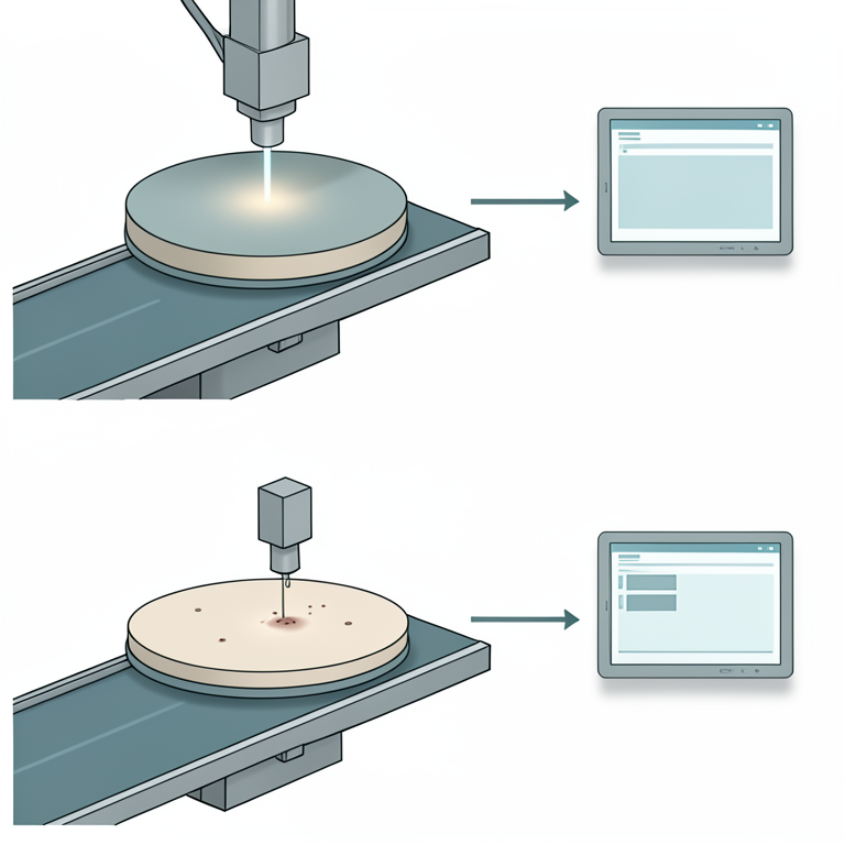
Decision Logic for ICV Control Chart Selection
AI-generated conceptual illustration (Industrial semiconductor wafers on a cleanroom conveyor belt). It explains the idea and does not show study data.
View source evidence ↗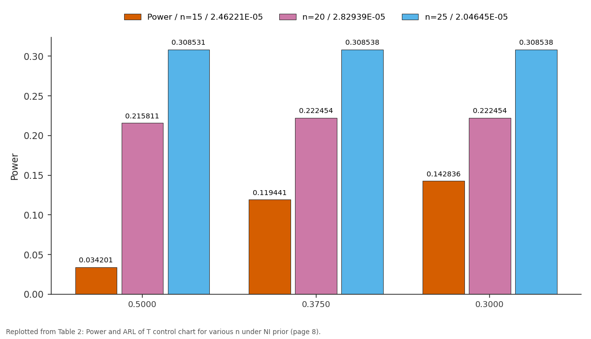
Power / n=15 / 2.46221E-05 and n=20 / 2.82939E-05 and more: 0.5000 vs 0.3750 vs 0.3000
Replotted from Table 2 (page 8) of the original paper. Every bar is the paper's own table value.
View source evidence ↗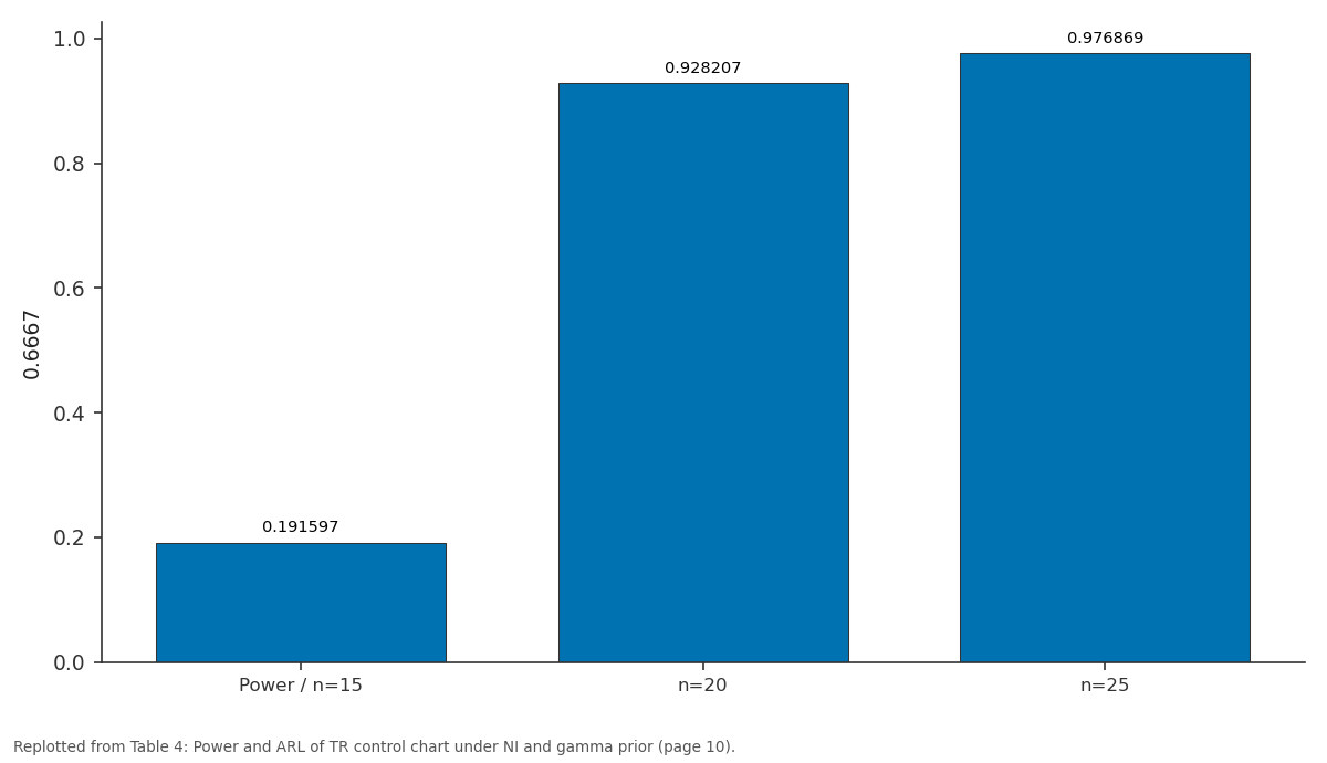
0.6667: Power / n=15 vs n=20 vs n=25
Replotted from Table 4 (page 10) of the original paper. Every bar is the paper's own table value.
View source evidence ↗Figures & tables
From the original paper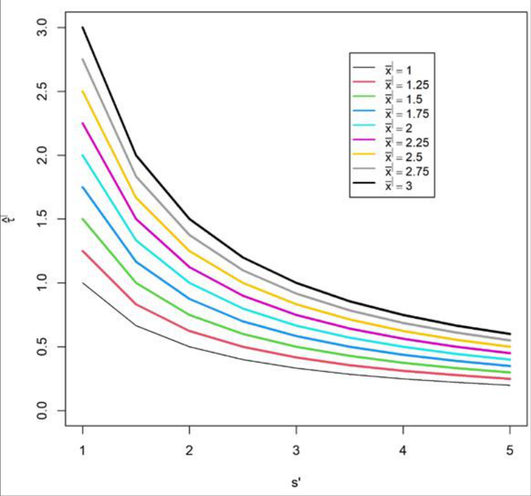 Figure 1
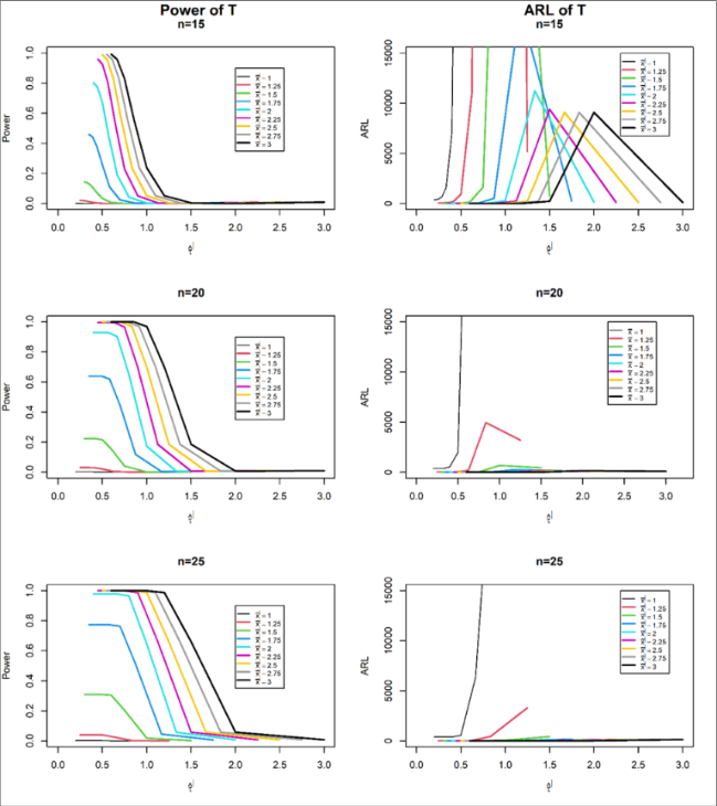 Figure 2
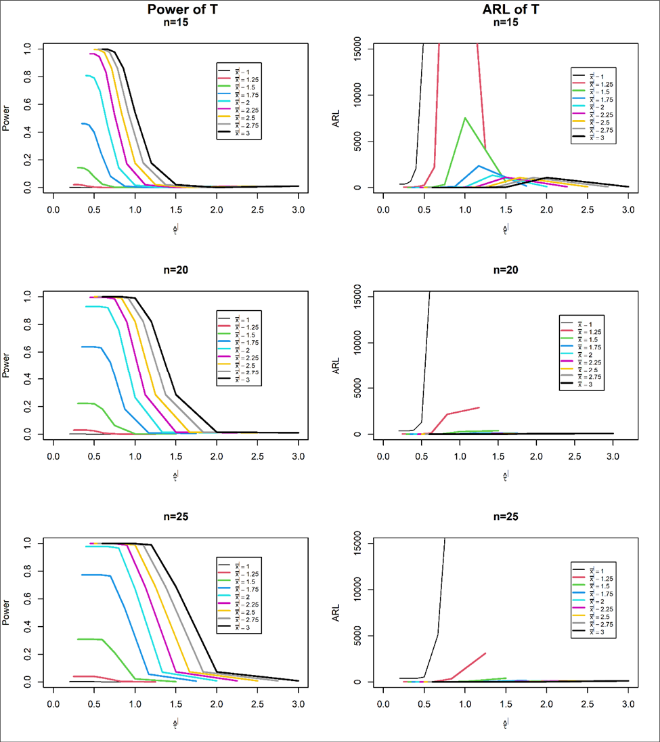 Figure 3
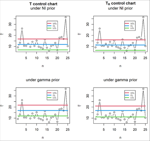 Figure 4
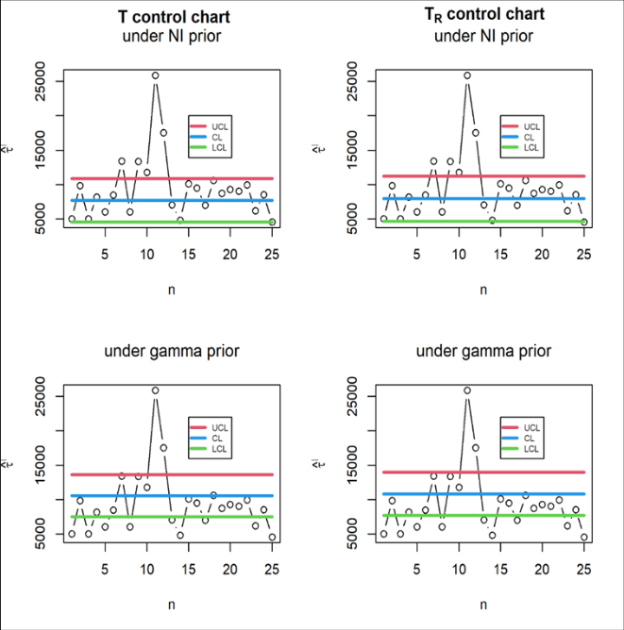 Figure 5
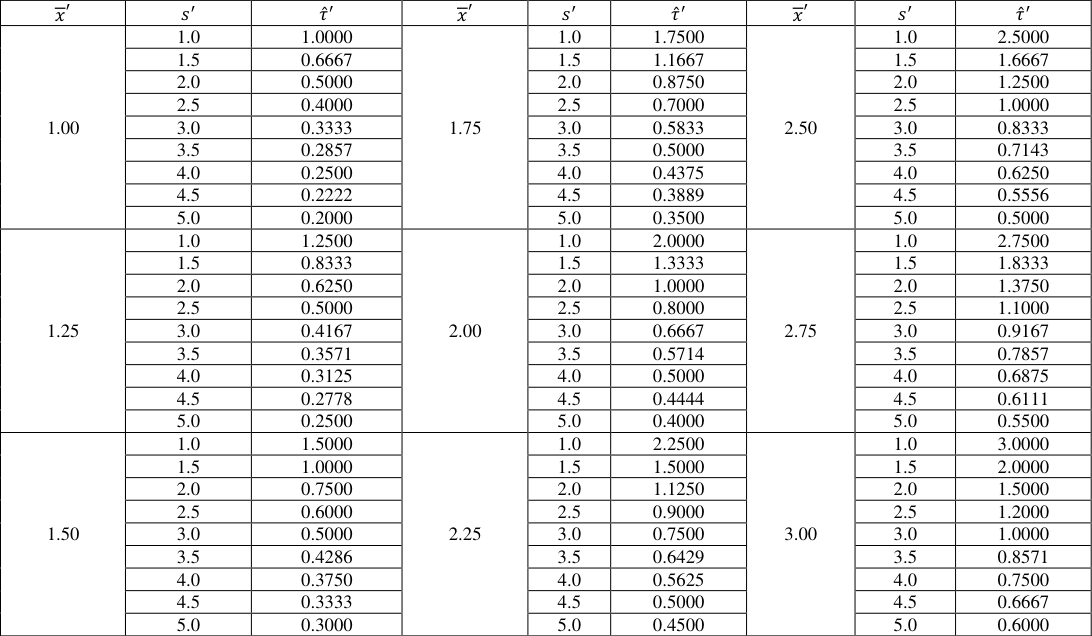 Table 1
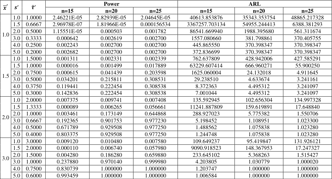 Table 2
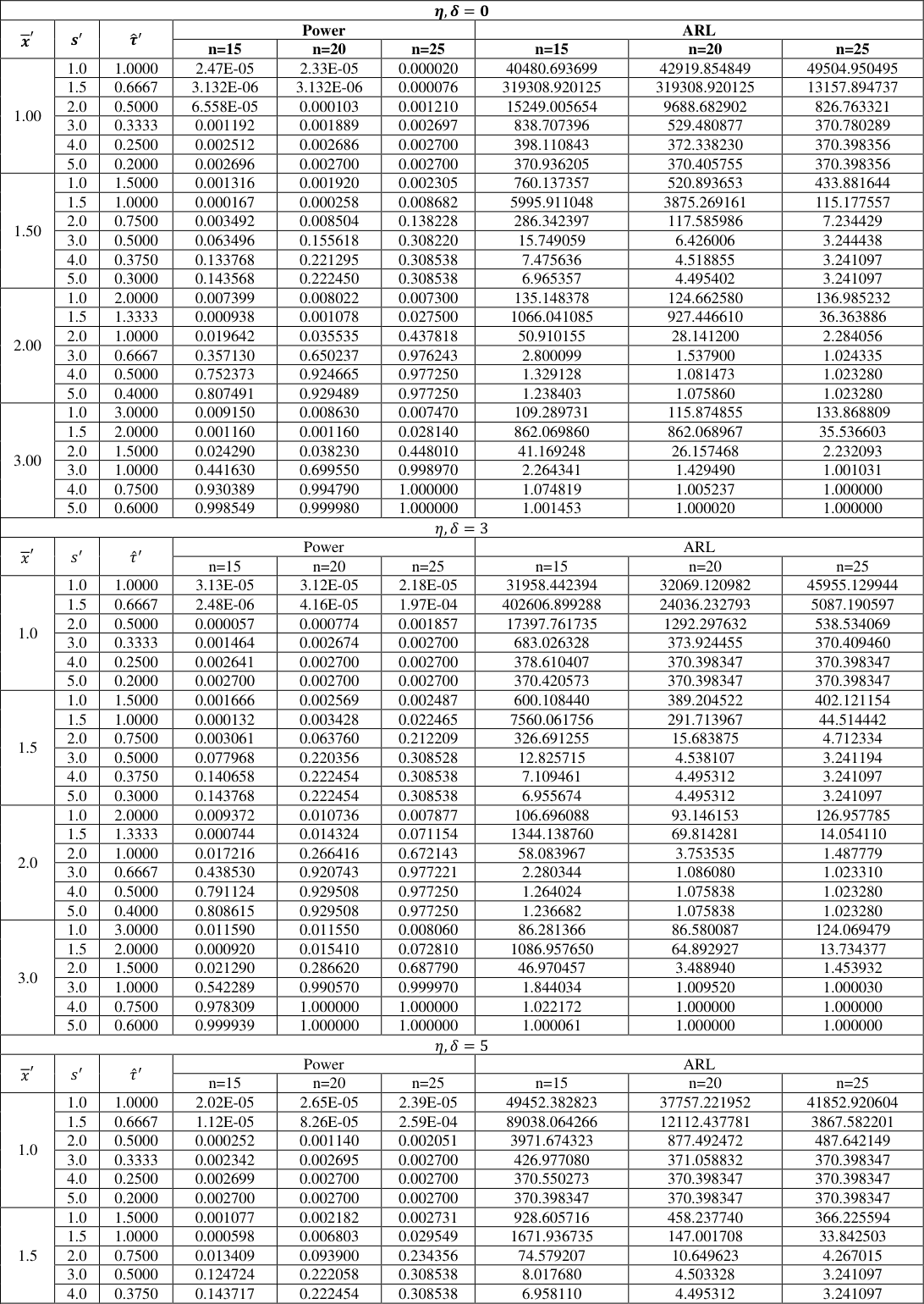 Table 3
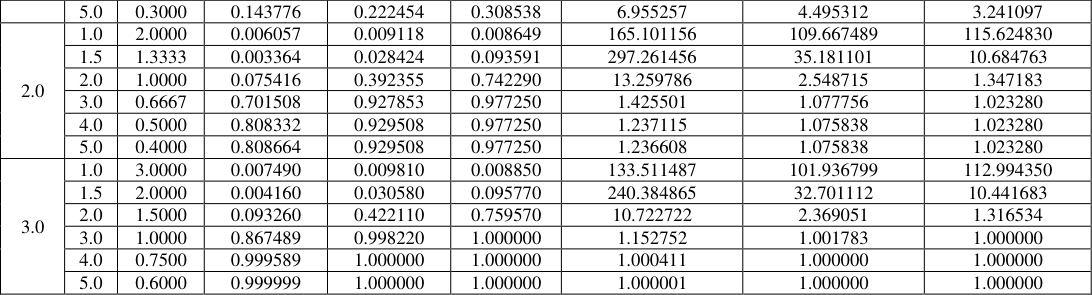 Table 4
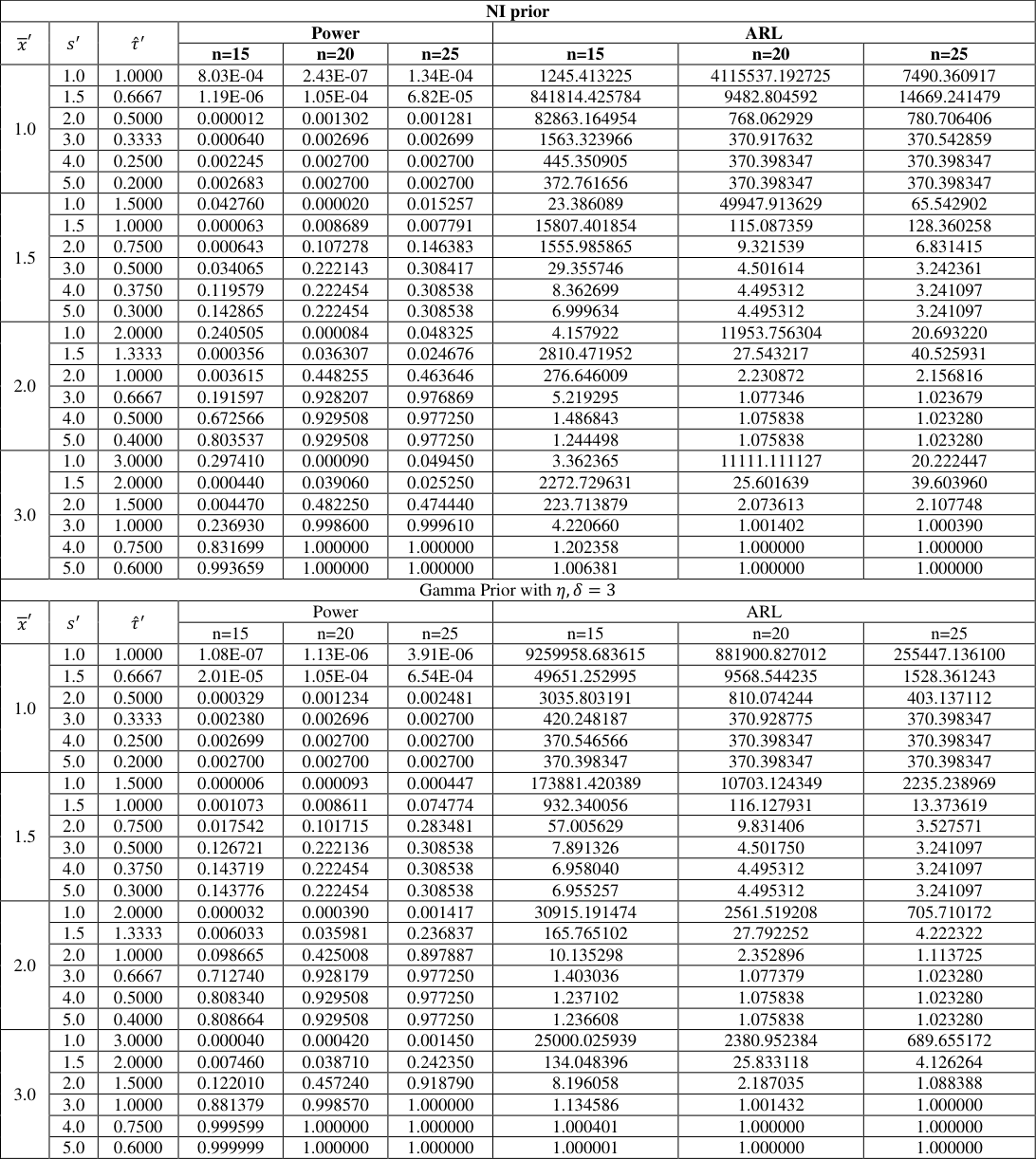 Table 4
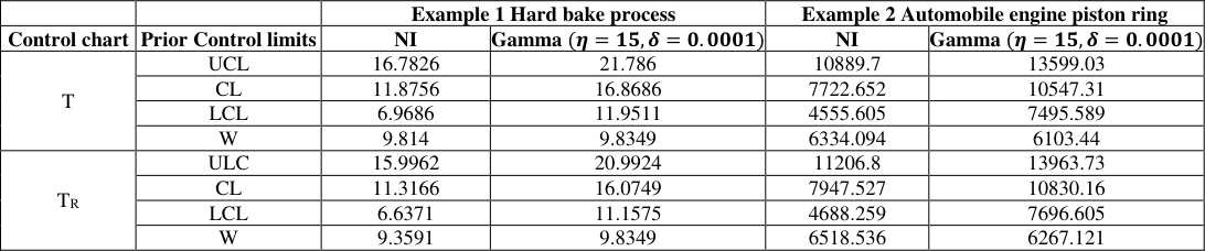 Table 5
Introduction
Process variation plays a prime role in process monitoring. Hence monitoring process variation using control charts is inevitable in manufacturing. Sometimes, quality practitioners are interested in calibrating relative change in process variance with respect to process mean known as CV which is unit free. The reciprocal of CV is ICV and it accounts for the measure of precision. The population ICV is given by 𝜏 = 𝜇 𝜎 (1) where 𝜇 is population mean and 𝜎 is population standard deviation (sd). The sample ICV is given by 𝜏̂= 𝑥 𝑠 (2) where 𝑥 = is sample sd. The control chart for ICV is helpful in maintaining quality of certain production processes such as manufacturing of surgical instruments, footwear, gems and jewelry, apparel, etc. Singh (1993) [9] studied the behavior of population ICV when a random sample of size n is drawn from various distributions including life testing distributions. Sharma and Krishna (1994) [8] constructed asymptotic distribution of sample ICV. Van Zyl and Van der Merwe (2017) [11] developed Bayesian procedure of obtaining control limits for CV using reference and probability matching priors. Kalkur and Rao (2017) [6] developed Bayes estimators for CV and ICV under normal model using various priors. Using Bayesian approach, the control charts were developed under conjugate priors for process average and process variance respectively by Bhat and Gokhale (2014a) and (2014b) [1][2] . These authors developed control chart for process sd using noninformative (NI), conjugate and non-conjugate priors in 2016. Bhat and Malagavi (2021a) [4] and (2021b) [5] respectively developed range based posterior control charts for process average and process variation.
In this paper, we focus on the development of Bayesian control charts for ICV under normal model. We use NI and gamma priors. In section 2, we obtain 𝐸(𝜏), 𝑉(𝜏), 𝐸(𝜏 𝑟 ), 𝑉(𝜏 𝑟 ) and construct control charts for ICV. We evaluate the performance of the proposed control charts using power and average run length (ARL) in section 3 and illustrate them with examples in section 4. Conclusions are given in section 5. Tables supporting our study are given in appendix.
Bayesian control charts for ICV
In this section, we derive posterior joint distribution of (𝜇, 1 𝜎 2 ) and propose posterior control charts (T and T R control charts) for ICV. We find 𝐸(𝜏), 𝑉(𝜏), 𝐸(𝜏 𝑟 ) and 𝑉(𝜏 𝑟 ) using joint posterior distribution of 𝜇 and 1 𝜎 2 under NI and gamma priors. Let X 1 , X 2 ,… X n be a random sample of size n from normal distribution with mean 𝜇 and variance 𝜎 2 . Then the likelihood function is given by
Assuming the prior distribution for 𝜇 as 𝜋(𝜇) = 1, the posterior distribution of 𝜇 is given by
𝑛
Hence, the probability density function of
We derive the posterior distribution of (
The posterior distribution of ( 1 𝜎 2 |𝑠 2 ) under NI prior is given by
Also, the posterior distribution of ( 1 𝜎 2 |𝑠 2 ) under gamma prior is given by
Since 𝜇 and 𝜎 2 are independent, the posterior joint distribution of (𝜇, 1 𝜎 2 ) is written as
Using (12), under NI prior,
Also, under gamma prior, using (13), we get
The proposed T control chart for ICV is given by 𝐿𝐶𝐿 𝑇 = 𝐸(𝜏) -3√𝑉(𝜏), 𝐶𝐿 𝑇 = 𝐸(𝜏) and 𝑈𝐶𝐿 𝑇 = 𝐸(𝜏) + 3√𝑉(𝜏).
where 𝐿𝐶𝐿 𝑇 is lower control limit, 𝑈𝐶𝐿 𝑇 is upper control limit and 𝐶𝐿 𝑇 is central line of T control chart. Under NI prior, the control chart is given by substituting ( 14), (15) in (18) and under gamma prior by substituting ( 16), (17) in (18). Further the width, W T of the T control chart is given by
When sample information is available in terms of extreme observations, the range is 𝑟 = 𝑥 (𝑛) -𝑥 (1) where 𝑥 (𝑛) and 𝑥 (1) are respectively the highest and lowest values of the data. According to Tippett (1925) in appropriate equations. Also, we obtain range based T R control chart and its width using 𝐸(𝜏 𝑟 ) and 𝑉(𝜏 𝑟 ).
Performance of the proposed control charts
In this section, we investigate the performance of the proposed T and T R control charts for ICV in terms of power and ARL. The power and ARL of any control chart is given by
where 𝛽 is probability of not detecting the shift in 𝜏̂′, where 𝜏̂′ = 𝑥 ′ 𝑠 ′ , 𝑥 ′ = 𝑥 + 𝑎 and 𝑠 ′ = 𝑠 + 𝑏, 𝑎 and 𝑏 are non-negative constants.
Under NI and gamma prior, 𝛽 of T control chart is respectively given by
Using (20) , we compute power and ARL of T control chart for various values of 𝜏̂′and n. In table 1, we provide values of 𝜏̂′ which are computed for various values of 𝑥 ′ and 𝑠 ′ . Here, 𝑥 = 1, 𝑎 = 0 (0.25) 2, 𝑠 = 1 and 𝑏 = 0 (0.5) 4. The values of 𝜏̂′ for different shifts are plotted in figure 1 using table 1. For n=15, 20, 25, power and ARL of T control chart under NI prior are given in table 2 and plotted in figure 2. Also, under gamma prior, for hyper parameters 𝜂 = 𝛿 = 0,3,5 the corresponding power, ARL values are given in tables 3. Using table 3 power and ARL of T control chart are plotted in figure 3 for 𝜂, 𝛿 = 3. Table 4 consists of power and ARL of T R control chart under NI prior and gamma prior with 𝜂, 𝛿 = 3. In these tables 10𝐸 -𝑙 represents 𝑒 -𝑙 , where 𝑙 is an integer.
| NI prior | — | — | — | — | — | — | — | — |
|---|---|---|---|---|---|---|---|---|
| 𝑥′ | 𝑠′ | 𝜏̂′ | Power | ARL | ||||
| n=15 | n=20 | n=25 | n=15 | n=20 | n=25 | |||
| 1.0 | 1.0 | 1.0000 | 8.03E-04 | 2.43E-07 | 1.34E-04 | 1245.413225 | 4115537.192725 | 7490.360917 |
| 1.5 | 0.6667 | 1.19E-06 | 1.05E-04 | 6.82E-05 | 841814.425784 | 9482.804592 | 14669.241479 | |
| 2.0 | 0.5000 | 0.000012 | 0.001302 | 0.001281 | 82863.164954 | 768.062929 | 780.706406 | |
| 3.0 | 0.3333 | 0.000640 | 0.002696 | 0.002699 | 1563.323966 | 370.917632 | 370.542859 | |
| 4.0 | 0.2500 | 0.002245 | 0.002700 | 0.002700 | 445.350905 | 370.398347 | 370.398347 | |
| 5.0 | 0.2000 | 0.002683 | 0.002700 | 0.002700 | 372.761656 | 370.398347 | 370.398347 | |
| 1.5 | 1.0 | 1.5000 | 0.042760 | 0.000020 | 0.015257 | 23.386089 | 49947.913629 | 65.542902 |
| 1.5 | 1.0000 | 0.000063 | 0.008689 | 0.007791 | 15807.401854 | 115.087359 | 128.360258 | |
| 2.0 | 0.7500 | 0.000643 | 0.107278 | 0.146383 | 1555.985865 | 9.321539 | 6.831415 | |
| 3.0 | 0.5000 | 0.034065 | 0.222143 | 0.308417 | 29.355746 | 4.501614 | 3.242361 | |
| 4.0 | 0.3750 | 0.119579 | 0.222454 | 0.308538 | 8.362699 | 4.495312 | 3.241097 | |
| 5.0 | 0.3000 | 0.142865 | 0.222454 | 0.308538 | 6.999634 | 4.495312 | 3.241097 | |
| 2.0 | 1.0 | 2.0000 | 0.240505 | 0.000084 | 0.048325 | 4.157922 | 11953.756304 | 20.693220 |
| 1.5 | 1.3333 | 0.000356 | 0.036307 | 0.024676 | 2810.471952 | 27.543217 | 40.525931 | |
| 2.0 | 1.0000 | 0.003615 | 0.448255 | 0.463646 | 276.646009 | 2.230872 | 2.156816 | |
| 3.0 | 0.6667 | 0.191597 | 0.928207 | 0.976869 | 5.219295 | 1.077346 | 1.023679 | |
| 4.0 | 0.5000 | 0.672566 | 0.929508 | 0.977250 | 1.486843 | 1.075838 | 1.023280 | |
| 5.0 | 0.4000 | 0.803537 | 0.929508 | 0.977250 | 1.244498 | 1.075838 | 1.023280 | |
| 3.0 | 1.0 | 3.0000 | 0.297410 | 0.000090 | 0.049450 | 3.362365 | 11111.111127 | 20.222447 |
| 1.5 | 2.0000 | 0.000440 | 0.039060 | 0.025250 | 2272.729631 | 25.601639 | 39.603960 | |
| 2.0 | 1.5000 | 0.004470 | 0.482250 | 0.474440 | 223.713879 | 2.073613 | 2.107748 | |
| 3.0 | 1.0000 | 0.236930 | 0.998600 | 0.999610 | 4.220660 | 1.001402 | 1.000390 | |
| 4.0 | 0.7500 | 0.831699 | 1.000000 | 1.000000 | 1.202358 | 1.000000 | 1.000000 | |
| 5.0 | 0.6000 | 0.993659 | 1.000000 | 1.000000 | 1.006381 | 1.000000 | 1.000000 | |
| Gamma Prior with 𝜂, 𝛿= 3 | ||||||||
| 𝑥′ | 𝑠′ | 𝜏̂′ | Power | ARL | ||||
| n=15 | n=20 | n=25 | n=15 | n=20 | n=25 | |||
| 1.0 | 1.0 | 1.0000 | 1.08E-07 | 1.13E-06 | 3.91E-06 | 9259958.683615 | 881900.827012 | 255447.136100 |
| 1.5 | 0.6667 | 2.01E-05 | 1.05E-04 | 6.54E-04 | 49651.252995 | 9568.544235 | 1528.361243 | |
| 2.0 | 0.5000 | 0.000329 | 0.001234 | 0.002481 | 3035.803191 | 810.074244 | 403.137112 | |
| 3.0 | 0.3333 | 0.002380 | 0.002696 | 0.002700 | 420.248187 | 370.928775 | 370.398347 | |
| 4.0 | 0.2500 | 0.002699 | 0.002700 | 0.002700 | 370.546566 | 370.398347 | 370.398347 | |
| 5.0 | 0.2000 | 0.002700 | 0.002700 | 0.002700 | 370.398347 | 370.398347 | 370.398347 | |
| 1.5 | 1.0 | 1.5000 | 0.000006 | 0.000093 | 0.000447 | 173881.420389 | 10703.124349 | 2235.238969 |
| 1.5 | 1.0000 | 0.001073 | 0.008611 | 0.074774 | 932.340056 | 116.127931 | 13.373619 | |
| 2.0 | 0.7500 | 0.017542 | 0.101715 | 0.283481 | 57.005629 | 9.831406 | 3.527571 | |
| 3.0 | 0.5000 | 0.126721 | 0.222136 | 0.308538 | 7.891326 | 4.501750 | 3.241097 | |
| 4.0 | 0.3750 | 0.143719 | 0.222454 | 0.308538 | 6.958040 | 4.495312 | 3.241097 | |
| 5.0 | 0.3000 | 0.143776 | 0.222454 | 0.308538 | 6.955257 | 4.495312 | 3.241097 | |
| 2.0 | 1.0 | 2.0000 | 0.000032 | 0.000390 | 0.001417 | 30915.191474 | 2561.519208 | 705.710172 |
| 1.5 | 1.3333 | 0.006033 | 0.035981 | 0.236837 | 165.765102 | 27.792252 | 4.222322 | |
| 2.0 | 1.0000 | 0.098665 | 0.425008 | 0.897887 | 10.135298 | 2.352896 | 1.113725 | |
| 3.0 | 0.6667 | 0.712740 | 0.928179 | 0.977250 | 1.403036 | 1.077379 | 1.023280 | |
| 4.0 | 0.5000 | 0.808340 | 0.929508 | 0.977250 | 1.237102 | 1.075838 | 1.023280 | |
| 5.0 | 0.4000 | 0.808664 | 0.929508 | 0.977250 | 1.236608 | 1.075838 | 1.023280 | |
| 3.0 | 1.0 | 3.0000 | 0.000040 | 0.000420 | 0.001450 | 25000.025939 | 2380.952384 | 689.655172 |
| 1.5 | 2.0000 | 0.007460 | 0.038710 | 0.242350 | 134.048396 | 25.833118 | 4.126264 | |
| 2.0 | 1.5000 | 0.122010 | 0.457240 | 0.918790 | 8.196058 | 2.187035 | 1.088388 | |
| 3.0 | 1.0000 | 0.881379 | 0.998570 | 1.000000 | 1.134586 | 1.001432 | 1.000000 | |
| 4.0 | 0.7500 | 0.999599 | 1.000000 | 1.000000 | 1.000401 | 1.000000 | 1.000000 | |
| 5.0 | 0.6000 | 0.999999 | 1.000000 | 1.000000 | 1.000001 | 1.000000 | 1.000000 |
Table text extracted from the original PDF; superscript letters are shown inline. The original table image is below.
View original table image
| — | 5.0 | 0.3000 | 0.143776 | 0.222454 | 0.308538 | 6.955257 | 4.495312 | 3.241097 |
|---|---|---|---|---|---|---|---|---|
| 2.0 | 1.0 | 2.0000 | 0.006057 | 0.009118 | 0.008649 | 165.101156 | 109.667489 | 115.624830 |
| 1.5 | 1.3333 | 0.003364 | 0.028424 | 0.093591 | 297.261456 | 35.181101 | 10.684763 | |
| 2.0 | 1.0000 | 0.075416 | 0.392355 | 0.742290 | 13.259786 | 2.548715 | 1.347183 | |
| 3.0 | 0.6667 | 0.701508 | 0.927853 | 0.977250 | 1.425501 | 1.077756 | 1.023280 | |
| 4.0 | 0.5000 | 0.808332 | 0.929508 | 0.977250 | 1.237115 | 1.075838 | 1.023280 | |
| 5.0 | 0.4000 | 0.808664 | 0.929508 | 0.977250 | 1.236608 | 1.075838 | 1.023280 | |
| 3.0 | 1.0 | 3.0000 | 0.007490 | 0.009810 | 0.008850 | 133.511487 | 101.936799 | 112.994350 |
| 1.5 | 2.0000 | 0.004160 | 0.030580 | 0.095770 | 240.384865 | 32.701112 | 10.441683 | |
| 2.0 | 1.5000 | 0.093260 | 0.422110 | 0.759570 | 10.722722 | 2.369051 | 1.316534 | |
| 3.0 | 1.0000 | 0.867489 | 0.998220 | 1.000000 | 1.152752 | 1.001783 | 1.000000 | |
| 4.0 | 0.7500 | 0.999589 | 1.000000 | 1.000000 | 1.000411 | 1.000000 | 1.000000 | |
| 5.0 | 0.6000 | 0.999999 | 1.000000 | 1.000000 | 1.000001 | 1.000000 | 1.000000 |
Table text extracted from the original PDF; superscript letters are shown inline. The original table image is below.
View original table image
| 𝜼, 𝜹= 𝟎 | — | — | — | — | — | — | — | — |
|---|---|---|---|---|---|---|---|---|
| 𝒙′ | 𝒔′ | 𝝉̂′ | Power | ARL | ||||
| n=15 | n=20 | n=25 | n=15 | n=20 | n=25 | |||
| 1.00 | 1.0 | 1.0000 | 2.47E-05 | 2.33E-05 | 0.000020 | 40480.693699 | 42919.854849 | 49504.950495 |
| 1.5 | 0.6667 | 3.132E-06 | 3.132E-06 | 0.000076 | 319308.920125 | 319308.920125 | 13157.894737 | |
| 2.0 | 0.5000 | 6.558E-05 | 0.000103 | 0.001210 | 15249.005654 | 9688.682902 | 826.763321 | |
| 3.0 | 0.3333 | 0.001192 | 0.001889 | 0.002697 | 838.707396 | 529.480877 | 370.780289 | |
| 4.0 | 0.2500 | 0.002512 | 0.002686 | 0.002700 | 398.110843 | 372.338230 | 370.398356 | |
| 5.0 | 0.2000 | 0.002696 | 0.002700 | 0.002700 | 370.936205 | 370.405755 | 370.398356 | |
| 1.50 | 1.0 | 1.5000 | 0.001316 | 0.001920 | 0.002305 | 760.137357 | 520.893653 | 433.881644 |
| 1.5 | 1.0000 | 0.000167 | 0.000258 | 0.008682 | 5995.911048 | 3875.269161 | 115.177557 | |
| 2.0 | 0.7500 | 0.003492 | 0.008504 | 0.138228 | 286.342397 | 117.585986 | 7.234429 | |
| 3.0 | 0.5000 | 0.063496 | 0.155618 | 0.308220 | 15.749059 | 6.426006 | 3.244438 | |
| 4.0 | 0.3750 | 0.133768 | 0.221295 | 0.308538 | 7.475636 | 4.518855 | 3.241097 | |
| 5.0 | 0.3000 | 0.143568 | 0.222450 | 0.308538 | 6.965357 | 4.495402 | 3.241097 | |
| 2.00 | 1.0 | 2.0000 | 0.007399 | 0.008022 | 0.007300 | 135.148378 | 124.662580 | 136.985232 |
| 1.5 | 1.3333 | 0.000938 | 0.001078 | 0.027500 | 1066.041085 | 927.446610 | 36.363886 | |
| 2.0 | 1.0000 | 0.019642 | 0.035535 | 0.437818 | 50.910155 | 28.141200 | 2.284056 | |
| 3.0 | 0.6667 | 0.357130 | 0.650237 | 0.976243 | 2.800099 | 1.537900 | 1.024335 | |
| 4.0 | 0.5000 | 0.752373 | 0.924665 | 0.977250 | 1.329128 | 1.081473 | 1.023280 | |
| 5.0 | 0.4000 | 0.807491 | 0.929489 | 0.977250 | 1.238403 | 1.075860 | 1.023280 | |
| 3.00 | 1.0 | 3.0000 | 0.009150 | 0.008630 | 0.007470 | 109.289731 | 115.874855 | 133.868809 |
| 1.5 | 2.0000 | 0.001160 | 0.001160 | 0.028140 | 862.069860 | 862.068967 | 35.536603 | |
| 2.0 | 1.5000 | 0.024290 | 0.038230 | 0.448010 | 41.169248 | 26.157468 | 2.232093 | |
| 3.0 | 1.0000 | 0.441630 | 0.699550 | 0.998970 | 2.264341 | 1.429490 | 1.001031 | |
| 4.0 | 0.7500 | 0.930389 | 0.994790 | 1.000000 | 1.074819 | 1.005237 | 1.000000 | |
| 5.0 | 0.6000 | 0.998549 | 0.999980 | 1.000000 | 1.001453 | 1.000020 | 1.000000 | |
| 𝜂, 𝛿= 3 | ||||||||
| 𝑥′ | 𝑠′ | 𝜏̂′ | Power | ARL | ||||
| n=15 | n=20 | n=25 | n=15 | n=20 | n=25 | |||
| 1.0 | 1.0 | 1.0000 | 3.13E-05 | 3.12E-05 | 2.18E-05 | 31958.442394 | 32069.120982 | 45955.129944 |
| 1.5 | 0.6667 | 2.48E-06 | 4.16E-05 | 1.97E-04 | 402606.899288 | 24036.232793 | 5087.190597 | |
| 2.0 | 0.5000 | 0.000057 | 0.000774 | 0.001857 | 17397.761735 | 1292.297632 | 538.534069 | |
| 3.0 | 0.3333 | 0.001464 | 0.002674 | 0.002700 | 683.026328 | 373.924455 | 370.409460 | |
| 4.0 | 0.2500 | 0.002641 | 0.002700 | 0.002700 | 378.610407 | 370.398347 | 370.398347 | |
| 5.0 | 0.2000 | 0.002700 | 0.002700 | 0.002700 | 370.420573 | 370.398347 | 370.398347 | |
| 1.5 | 1.0 | 1.5000 | 0.001666 | 0.002569 | 0.002487 | 600.108440 | 389.204522 | 402.121154 |
| 1.5 | 1.0000 | 0.000132 | 0.003428 | 0.022465 | 7560.061756 | 291.713967 | 44.514442 | |
| 2.0 | 0.7500 | 0.003061 | 0.063760 | 0.212209 | 326.691255 | 15.683875 | 4.712334 | |
| 3.0 | 0.5000 | 0.077968 | 0.220356 | 0.308528 | 12.825715 | 4.538107 | 3.241194 | |
| 4.0 | 0.3750 | 0.140658 | 0.222454 | 0.308538 | 7.109461 | 4.495312 | 3.241097 | |
| 5.0 | 0.3000 | 0.143768 | 0.222454 | 0.308538 | 6.955674 | 4.495312 | 3.241097 | |
| 2.0 | 1.0 | 2.0000 | 0.009372 | 0.010736 | 0.007877 | 106.696088 | 93.146153 | 126.957785 |
| 1.5 | 1.3333 | 0.000744 | 0.014324 | 0.071154 | 1344.138760 | 69.814281 | 14.054110 | |
| 2.0 | 1.0000 | 0.017216 | 0.266416 | 0.672143 | 58.083967 | 3.753535 | 1.487779 | |
| 3.0 | 0.6667 | 0.438530 | 0.920743 | 0.977221 | 2.280344 | 1.086080 | 1.023310 | |
| 4.0 | 0.5000 | 0.791124 | 0.929508 | 0.977250 | 1.264024 | 1.075838 | 1.023280 | |
| 5.0 | 0.4000 | 0.808615 | 0.929508 | 0.977250 | 1.236682 | 1.075838 | 1.023280 | |
| 3.0 | 1.0 | 3.0000 | 0.011590 | 0.011550 | 0.008060 | 86.281366 | 86.580087 | 124.069479 |
| 1.5 | 2.0000 | 0.000920 | 0.015410 | 0.072810 | 1086.957650 | 64.892927 | 13.734377 | |
| 2.0 | 1.5000 | 0.021290 | 0.286620 | 0.687790 | 46.970457 | 3.488940 | 1.453932 | |
| 3.0 | 1.0000 | 0.542289 | 0.990570 | 0.999970 | 1.844034 | 1.009520 | 1.000030 | |
| 4.0 | 0.7500 | 0.978309 | 1.000000 | 1.000000 | 1.022172 | 1.000000 | 1.000000 | |
| 5.0 | 0.6000 | 0.999939 | 1.000000 | 1.000000 | 1.000061 | 1.000000 | 1.000000 | |
| 𝜂, 𝛿= 5 | ||||||||
| 𝑥′ | 𝑠′ | 𝜏̂′ | Power | ARL | ||||
| n=15 | n=20 | n=25 | n=15 | n=20 | n=25 | |||
| 1.0 | 1.0 | 1.0000 | 2.02E-05 | 2.65E-05 | 2.39E-05 | 49452.382823 | 37757.221952 | 41852.920604 |
| 1.5 | 0.6667 | 1.12E-05 | 8.26E-05 | 2.59E-04 | 89038.064266 | 12112.437781 | 3867.582201 | |
| 2.0 | 0.5000 | 0.000252 | 0.001140 | 0.002051 | 3971.674323 | 877.492472 | 487.642149 | |
| 3.0 | 0.3333 | 0.002342 | 0.002695 | 0.002700 | 426.977080 | 371.058832 | 370.398347 | |
| 4.0 | 0.2500 | 0.002699 | 0.002700 | 0.002700 | 370.550273 | 370.398347 | 370.398347 | |
| 5.0 | 0.2000 | 0.002700 | 0.002700 | 0.002700 | 370.398347 | 370.398347 | 370.398347 | |
| 1.5 | 1.0 | 1.5000 | 0.001077 | 0.002182 | 0.002731 | 928.605716 | 458.237740 | 366.225594 |
| 1.5 | 1.0000 | 0.000598 | 0.006803 | 0.029549 | 1671.936735 | 147.001708 | 33.842503 | |
| 2.0 | 0.7500 | 0.013409 | 0.093900 | 0.234356 | 74.579207 | 10.649623 | 4.267015 | |
| 3.0 | 0.5000 | 0.124724 | 0.222058 | 0.308538 | 8.017680 | 4.503328 | 3.241097 | |
| 4.0 | 0.3750 | 0.143717 | 0.222454 | 0.308538 | 6.958110 | 4.495312 | 3.241097 |
Table text extracted from the original PDF; superscript letters are shown inline. The original table image is below.
View original table image
| 𝒙′ | 𝒔′ | 𝝉̂′ | Power | — | — | ARL | — | — |
|---|---|---|---|---|---|---|---|---|
| n=15 | n=20 | n=25 | n=15 | n=20 | n=25 | |||
| 1.0 | 1.0 | 1.0000 | 2.46221E-05 | 2.82939E-05 | 2.04645E-05 | 40613.853876 | 35343.353754 | 48865.217328 |
| 1.5 | 0.6667 | 2.96978E-07 | 1.81966E-05 | 0.000156534 | 3367257.703134 | 54955.244413 | 6388.381293 | |
| 2.0 | 0.5000 | 1.15551E-05 | 0.000503 | 0.001782 | 86541.669940 | 1988.395680 | 561.311674 | |
| 3.0 | 0.3333 | 0.000642 | 0.002619 | 0.002700 | 1557.080660 | 381.798861 | 370.405755 | |
| 4.0 | 0.2500 | 0.002243 | 0.002700 | 0.002700 | 445.865550 | 370.398347 | 370.398347 | |
| 5.0 | 0.2000 | 0.002682 | 0.002700 | 0.002700 | 372.836699 | 370.398347 | 370.398347 | |
| 1.5 | 1.0 | 1.5000 | 0.001311 | 0.002331 | 0.002339 | 762.637809 | 428.942006 | 427.585291 |
| 1.5 | 1.0000 | 0.000016 | 0.001499 | 0.017889 | 63229.607414 | 666.960271 | 55.900250 | |
| 2.0 | 0.7500 | 0.000615 | 0.041439 | 0.203598 | 1625.060004 | 24.132018 | 4.911645 | |
| 3.0 | 0.5000 | 0.034201 | 0.215811 | 0.308531 | 29.238510 | 4.633674 | 3.241161 | |
| 4.0 | 0.3750 | 0.119441 | 0.222454 | 0.308538 | 8.372363 | 4.495312 | 3.241097 | |
| 5.0 | 0.3000 | 0.142836 | 0.222454 | 0.308538 | 7.001044 | 4.495312 | 3.241097 | |
| 2.0 | 1.0 | 2.0000 | 0.007375 | 0.009741 | 0.007408 | 135.592945 | 102.656304 | 134.997328 |
| 1.5 | 1.3333 | 0.000089 | 0.006265 | 0.056661 | 11241.887809 | 159.619891 | 17.648840 | |
| 2.0 | 1.0000 | 0.003461 | 0.173149 | 0.644868 | 288.927023 | 5.775382 | 1.550706 | |
| 3.0 | 0.6667 | 0.192365 | 0.901753 | 0.977230 | 5.198452 | 1.108951 | 1.023300 | |
| 4.0 | 0.5000 | 0.671789 | 0.929508 | 0.977250 | 1.488562 | 1.075838 | 1.023280 | |
| 5.0 | 0.4000 | 0.803375 | 0.929508 | 0.977250 | 1.244748 | 1.075838 | 1.023280 | |
| 3.0 | 1.0 | 3.0000 | 0.009120 | 0.010480 | 0.007580 | 109.649237 | 95.419847 | 131.926121 |
| 1.5 | 2.0000 | 0.000110 | 0.006740 | 0.057980 | 9090.918523 | 148.367953 | 17.247327 | |
| 2.0 | 1.5000 | 0.004280 | 0.186280 | 0.659880 | 233.645102 | 5.368263 | 1.515427 | |
| 3.0 | 1.0000 | 0.237880 | 0.970140 | 0.999980 | 4.203805 | 1.030779 | 1.000020 | |
| 4.0 | 0.7500 | 0.830739 | 1.000000 | 1.000000 | 1.203747 | 1.000000 | 1.000000 | |
| 5.0 | 0.6000 | 0.993459 | 1.000000 | 1.000000 | 1.006584 | 1.000000 | 1.000000 |
Table text extracted from the original PDF; superscript letters are shown inline. The original table image is below.
View original table image
| 𝑥′ | 𝑠′ | 𝜏̂′ | 𝑥′ | 𝑠′ | 𝜏̂′ | 𝑥′ | 𝑠′ | 𝜏̂′ |
|---|---|---|---|---|---|---|---|---|
| 1.00 | 1.0 | 1.0000 | 1.75 | 1.0 | 1.7500 | 2.50 | 1.0 | 2.5000 |
| 1.5 | 0.6667 | 1.5 | 1.1667 | 1.5 | 1.6667 | |||
| 2.0 | 0.5000 | 2.0 | 0.8750 | 2.0 | 1.2500 | |||
| 2.5 | 0.4000 | 2.5 | 0.7000 | 2.5 | 1.0000 | |||
| 3.0 | 0.3333 | 3.0 | 0.5833 | 3.0 | 0.8333 | |||
| 3.5 | 0.2857 | 3.5 | 0.5000 | 3.5 | 0.7143 | |||
| 4.0 | 0.2500 | 4.0 | 0.4375 | 4.0 | 0.6250 | |||
| 4.5 | 0.2222 | 4.5 | 0.3889 | 4.5 | 0.5556 | |||
| 5.0 | 0.2000 | 5.0 | 0.3500 | 5.0 | 0.5000 | |||
| 1.25 | 1.0 | 1.2500 | 2.00 | 1.0 | 2.0000 | 2.75 | 1.0 | 2.7500 |
| 1.5 | 0.8333 | 1.5 | 1.3333 | 1.5 | 1.8333 | |||
| 2.0 | 0.6250 | 2.0 | 1.0000 | 2.0 | 1.3750 | |||
| 2.5 | 0.5000 | 2.5 | 0.8000 | 2.5 | 1.1000 | |||
| 3.0 | 0.4167 | 3.0 | 0.6667 | 3.0 | 0.9167 | |||
| 3.5 | 0.3571 | 3.5 | 0.5714 | 3.5 | 0.7857 | |||
| 4.0 | 0.3125 | 4.0 | 0.5000 | 4.0 | 0.6875 | |||
| 4.5 | 0.2778 | 4.5 | 0.4444 | 4.5 | 0.6111 | |||
| 5.0 | 0.2500 | 5.0 | 0.4000 | 5.0 | 0.5500 | |||
| 1.50 | 1.0 | 1.5000 | 2.25 | 1.0 | 2.2500 | 3.00 | 1.0 | 3.0000 |
| 1.5 | 1.0000 | 1.5 | 1.5000 | 1.5 | 2.0000 | |||
| 2.0 | 0.7500 | 2.0 | 1.1250 | 2.0 | 1.5000 | |||
| 2.5 | 0.6000 | 2.5 | 0.9000 | 2.5 | 1.2000 | |||
| 3.0 | 0.5000 | 3.0 | 0.7500 | 3.0 | 1.0000 | |||
| 3.5 | 0.4286 | 3.5 | 0.6429 | 3.5 | 0.8571 | |||
| 4.0 | 0.3750 | 4.0 | 0.5625 | 4.0 | 0.7500 | |||
| 4.5 | 0.3333 | 4.5 | 0.5000 | 4.5 | 0.6667 | |||
| 5.0 | 0.3000 | 5.0 | 0.4500 | 5.0 | 0.6000 |
Table text extracted from the original PDF; superscript letters are shown inline. The original table image is below.
View original table image
From figure 2 and table 2, it is seen that, for a given value of n, power increases as 𝑥 ′ increases and decreases as 𝜏̂′ increases.
Also, for a specified value of 𝜏̂′, power increases as n increases. For all the values of 𝑥 ′ , for n=15 and increasing 𝜏̂′, ARL increases up to some value of 𝜏̂′ and then decreases. But for n=20, 25, ARL increases as 𝜏̂′ increases for different values of 𝑥 ′ .
From figure 3 and table 3, it is noticed that, for a given value of n, power increases as 𝑥 ′ increases and decreases as 𝜏̂′ increases.
Also, for a specified value of 𝜏̂′, power increases as n increases. For all the values of 𝑥 ′ , for n=15, 20 and increasing 𝜏̂′, ARL increases up to some value of 𝜏̂′ and then decreases. But for n=25, ARL increases as 𝜏̂′ increases.
From tables 2 and 3 it is observed that, power of T control chart increases and ARL decreases with increasing values of n under both priors. Also, power of T control chart increases with increasing values of hyper parameters under gamma prior for a given shift in 𝜏. From table 4, it is found that, power of T R control chart increases with increasing values of n. On comparing T and T R control charts under NI and gamma priors, power of T R control chart is higher than power of T control chart. However, for smaller values of n, power and ARL of both T and T R control charts are almost equal. From figure 1 and table 1, we observe that, for a given value of 𝑠 ′ , 𝜏̂′ increases as 𝑥 ′ increases and decreases as 𝑠 ′ increases
Illustration
In this section, we illustrate the proposed T and T R control charts in figures 4 and 5 respectively for examples on hard bake process and automobile engine piston ring due to Montgomery (1996). Here, we make use of first twenty five data points of these data and compute 𝜏̂′ for each subgroup. Then 𝜏̂′ is plotted for various samples. The control limits and width of the control charts are provided in table 5. When subgroup size is 5, d=2.326 and we consider 𝜂 = 15, 𝛿 = 0.0001.
| — | — | Example 1 Hard bake process | — | Example 2 Automobile engine piston ring | — |
|---|---|---|---|---|---|
| Control chart | Prior Control limits | NI | Gamma (𝜼= 𝟏𝟓, 𝜹= 𝟎. 𝟎𝟎𝟎𝟏) | NI | Gamma (𝜼= 𝟏𝟓, 𝜹= 𝟎. 𝟎𝟎𝟎𝟏) |
| T | UCL | 16.7826 | 21.786 | 10889.7 | 13599.03 |
| CL | 11.8756 | 16.8686 | 7722.652 | 10547.31 | |
| LCL | 6.9686 | 11.9511 | 4555.605 | 7495.589 | |
| W | 9.814 | 9.8349 | 6334.094 | 6103.44 | |
| TR | ULC | 15.9962 | 20.9924 | 11206.8 | 13963.73 |
| CL | 11.3166 | 16.0749 | 7947.527 | 10830.16 | |
| LCL | 6.6371 | 11.1575 | 4688.259 | 7696.605 | |
| W | 9.3591 | 9.8349 | 6518.536 | 6267.121 |
Table text extracted from the original PDF; superscript letters are shown inline. The original table image is below.
View original table image
Example 1: Hard bake process
The data consists of 25 samples with each sample having subgroup of size 5. It is the measurement of flow width (in micron) in hard-bake process for semi-conductor manufacturing. From figure 4 and table 5, it is observed that, the control limits of T and T R control charts under NI prior are lower than that of gamma prior. Also, width under gamma prior is wider than width under NI prior. The width of T R control chart is narrower than width of T control chart under NI prior, whereas widths of both control charts are same under gamma prior.
Example 2: Automobile engine piston ring inside diameter
The data is on measurement of inside diameter (in mm) of piston rings for automobile engine. It contains 25 samples with each of size 5.
Figure 5: T and TR control charts for automobile engine piston ring data
From figure 5 and table 5, it is seen that, for T and T R control charts the control limits under gamma prior are higher than control limits under NI prior, but the width under gamma prior is narrower than width under NI prior. Also, width of T R control chart is wider than width of T control chart under both NI and gamma priors.
Conclusions
In this section, we record our conclusions about the proposed control charts for process ICV, 𝜏 = 𝜇 𝜎 , the process precision. Here 𝜇 is process mean and 𝜎 is process sd. A posterior control chart, that is, T control chart for process precision using Bayesian approach is proposed. The sample ICV is 𝜏̂= 𝑥 𝑠 where 𝑥 is sample mean and s is sample sd. Under NI and gamma priors, when process measurements follow normal distribution, the T control chart is developed. We obtain posterior joint distribution of (𝜇, 1 𝜎 2 |𝑠 2 ) under NI, gamma priors and derive 𝐸(𝜏), 𝑉(𝜏) under both priors. The control limits and width of T control chart are developed using 𝐸(𝜏), 𝑉(𝜏). For T control chart, under NI prior, for a given value of n, power increases as shift in 𝑥 increases and decreases as shift in 𝜏̂ increases. For a specified value of shift in 𝜏, power increases with increasing value of n and ARL increases with increasing shifts in 𝜏̂ and higher values of n. Under gamma prior, for increasing values of n, power increases with increasing shifts in 𝑥 when 𝜂 and 𝛿 take higher values.
For a given 𝜂, 𝛿 and n, the power decreases as shift in 𝜏̂ increases. On substituting 𝑠 = 𝑟 𝑑 , we obtain control limits based on range and develop T R control chart. The behavior of this control chart is similar to that of T control chart. T R control chart outperforms T control chart for moderate and large values of n. However, performance of both the control charts are the same for small values of n. In hard bake process data, under NI prior width of T control chart is wider than width of T R control chart and under gamma prior width of both control charts are same. Further, in automobile engine piston ring data, the width of T R control chart is wider than width of T control chart under both priors. T control chart is useful when process precision is of prime concern and practitioners have prior information about the process mean and variance, whereas, T R control chart is helpful when sample information is available in terms of extreme observations.
Appendix
Appendix
References
6 in the original paper- Bhat SV, Gokhale KD. Posterior Control Chart for Standard Deviation based on Conjugate Prior. Journal of Indian Statistical Association. 2016;54(1&2):157-166.
- Kalkur TA, Rao A. Bayes estimator for coefficient of variation and inverse coefficient of variation for the normal distribution. International Journal of Statistics and Systems. 2017;12(4):721-732.
- Sharma, Krishna. Asymptotic sampling distribution of inverse coefficient of variation and its applications. IEEE Transactions on Reliability. 1994;43(4):630-633.
- Singh M. Behavior of Sample Coefficient of Variation drawn from several distributions, Sankya, 55, series B., Pt 1. 1993. p. 65-76.
- Tippett LHC. On the extreme individuals and the range of samples taken from a normal population. Biometrika, 1925;17(1):364-387.
- Van Zyl R, Van der Merwe AJ. A Bayesian control chart for a common coefficient of variation, Communications in Statistics -Theory and Methods. 2017;46:12, 5795 5811, DOI: 10.1080/03610926.2015.1112914