
Research article · 2023 · Full text
International Journal of Statistics and Applied MathematicsTrends in total factor productivity of sugarcane in Maharashtra: A state level evidence using DEA and SFA approach
Volume 8(5S) · Pages 808–813 · DOI: 10.22271/maths.2023.v8.i5sl.1289 ↗
Research areasAgricultural Economics and PracticesEfficiency Analysis Using DEA
Abstract
Author-writtenThis paper applied the both parametric and non-parametric approaches of productivity estimation for sugarcane in Maharashtra for the period of 1980-81 to 2020-21. The result from both the approaches signifies the importance in shift due to technological adoption as a vital source of productivity growth. The estimation of DEA and SFA produced similar results at spatial and temporal directions thus validating the TFP estimation. The analysis for growth rate, instability and decomposition analysis has been carried out for five sub-periods as per the reforms in the sugarcane industry and overall period (1950-51 to 2020-21). The state is witnessing a positive growth rate in area, production and productivity after the Mature Economic Reforms after 1990’s. However the state is suffering from serious instability issues in the sub-periods IV and V due to the scarcity of water and decline in groundwater table of the state. The positive TFP growth has been associated with associated with 0.3 per cent and a declining mean technical efficiency by -0.1 per cent per year. The TFP revived by 1.09 percent after the reforms in the sugar industry. The estimated regression results for TFP determinants revealed pressure on irrigation facilities due to prolonged drought condition of state. Since sugarcane is the leading cash crop of the state and large revenue is being generated by the crop sugar mills, balanced nutrients, and rural literacy all of these have a positive and significant contribution in increasing the agricultural productivity of the state. The results have revealed the yield stagnation is not only due to technology fatigue, but could be due to slacked input intensification. An obvious extension of the study could be incorporating more crops and states for an exhaustive and comparative analysis.
Summary
Source-checkedPlain-language reading of the full paper, prepared with AI and checked against the text. Each point links to the authors' own words.
Why it matters
- Agricultural productivity is a critical factor for addressing rural poverty and ensuring food availability. View evidence ↗
- Sugarcane is a vital cash crop in India, with significant production levels in states like Uttar Pradesh. View evidence ↗
The question
- The study aims to analyze the trends and factors influencing the Total Factor Productivity (TFP) of sugarcane in Maharashtra. View evidence ↗
What they did
- The analysis was divided into five distinct sub-periods to track growth patterns in sugarcane production. View evidence ↗
- TFP determinants were analyzed using data on government spending for research and extension, irrigation percentages, rural literacy, and the number of sugar mills. View evidence ↗
What they found
- Sugarcane area showed a positive growth rate of 3.9% over the overall period, with specific sub-period rates ranging from 2.0% to 4.3%. View evidence ↗
- Production grew at an overall rate of 4.0%, peaking at 5.2% in sub-period II before dropping to an insignificant 0.6% in sub-period III. View evidence ↗
- Yield was the primary driver of production changes, contributing 95.49% in the overall period and peaking at 96% in sub-period IV. View evidence ↗
- The state experienced high instability in area (30.78%) and production (30.50%) over the overall period, and moderate instability in yield (13.06%). View evidence ↗
- Maximum Likelihood Estimation (MLE) indicated that while production inputs were positive, they were statistically insignificant at the 1% level. View evidence ↗
What it means
- The authors conclude that frequent droughts, water scarcity, and declining groundwater tables are the primary causes of yield instability. View evidence ↗
- The authors recommend developing input-responsive sugarcane varieties to improve crop efficiency and balance TFP contributions. View evidence ↗
- The authors suggest that future research should include more crops and states to provide a more exhaustive comparative analysis. View evidence ↗
Visual summary
3 visualsIllustrations explain the paper; charts are replotted from the paper's own table values.
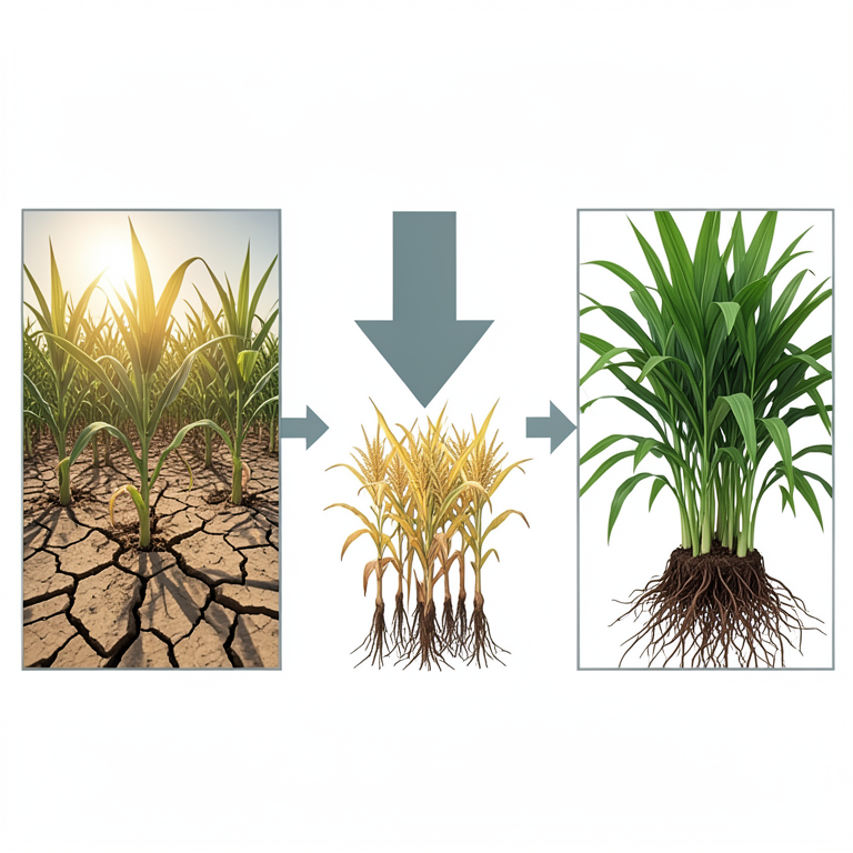
Factors Affecting Sugarcane Productivity
AI-generated conceptual illustration (Sugarcane plants in a field). It explains the idea and does not show study data.
View source evidence ↗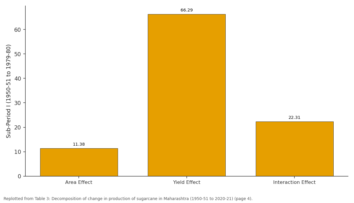
Sub-Period I (1950-51 to 1979-80): Area Effect vs Yield Effect vs Interaction Effect
Replotted from Table 3 (page 4) of the original paper. Every bar is the paper's own table value.
View source evidence ↗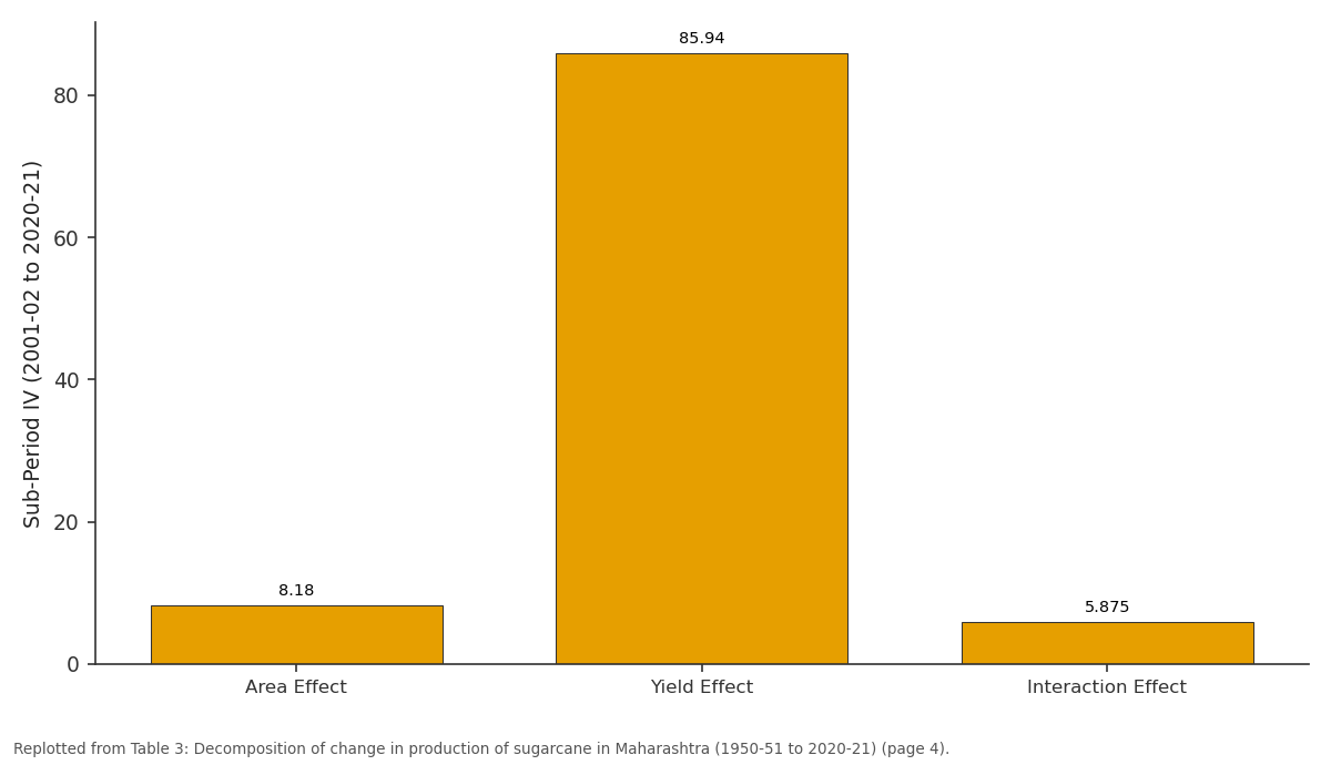
Sub-Period IV (2001-02 to 2020-21): Area Effect vs Yield Effect vs Interaction Effect
Replotted from Table 3 (page 4) of the original paper. Every bar is the paper's own table value.
View source evidence ↗Figures & tables
From the original paper Table 1
 Table 2
 Table 3
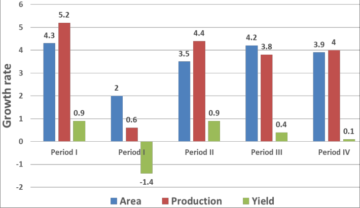 Figure 1
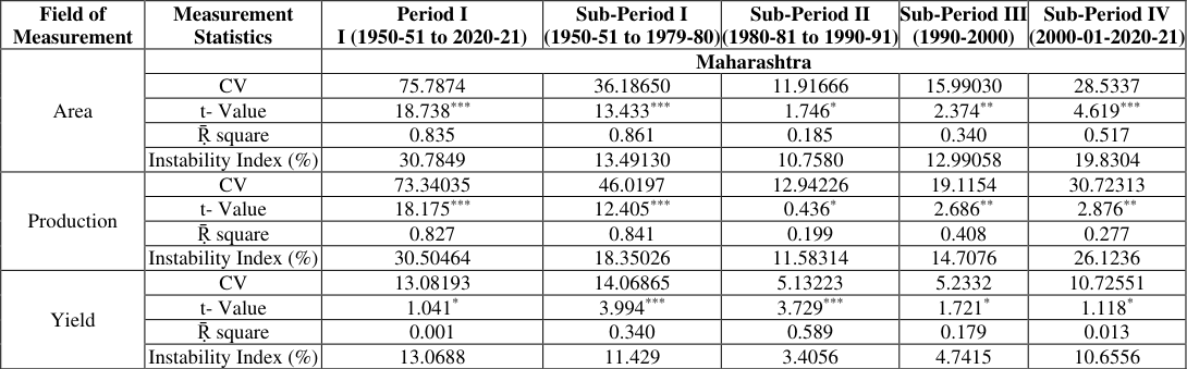 Table 4
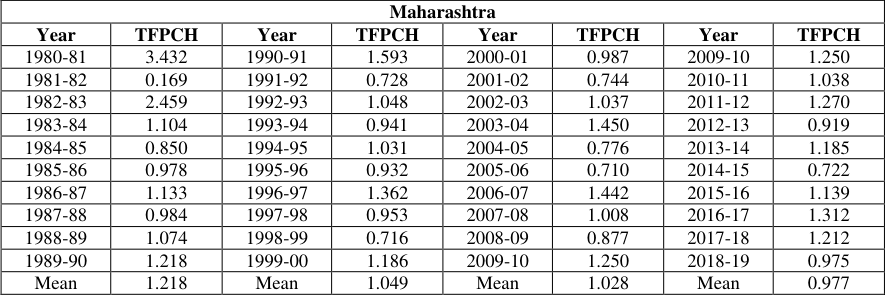 Table 5
 Table 6
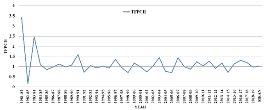 Figure 2
Introduction
The agricultural productivity always remains an important driver for the especial concerns such as food availability and rural poverty since the 1990s. The growth in the TFP promotes the rural sector to spend more on the non-farm sectors. This more specifically leads to the support the rural farm communities towards the non-farm commodities and service such as consumer goods and service, inputs and services to boost agricultural production, processing and marketing services. The slow agricultural growth could be due to reduce demand for food, slow technological change in agriculture, lack of employment opportunities for part time smallholders, limited technology adoption by full-time farmers. India is the largest consumer and the second-largest producer of sugar in the world after Brazil. Average annual production of sugarcane is around 35.5 crore tonnes which is used to produce around 3 crore tonnes of sugar. The domestic consumption is estimated to be around 2.6 crore tonnes in the current financial year. Sugarcane is one of the most important cash crop of Uttar Pradesh. It is the highest sugarcane producing State in sub-tropical zone having area about 22.77 lakh ha with the production of 135.64 Million tonne cane. About 50 million farmers and 3-5 lakhs skilled and unskilled workers are engaged in cultivation of sugarcane and sugar industries and its allied industries. There are few studies which have documented the total factor productivity of sugarcane using both the parametric and non-parametric approaches. This paper has looked upon the major trends and factors affecting TFP of the major cash crop of Maharashtra. Using the panel data for the time period (1980-81to 2020-2021), we have estimated parametric stochastic frontier analysis (SFA) (Aigner et al., 1977) [1] and non-parametric data envelopment analysis (DEA) (Charnes et al., 1978) [3] and discussed he results obtained from both the approaches. The purpose of using both the approaches was to counter verify the results obtained by one another. Using the Malmquist index (see Coelli and Rao, 2005 [6] for more details) non-parametric DEA can be used to decompose TFP growth into movements of the frontier and movement towards the frontier. On the other hand, the merit of SFA is that it considers stochastic noise in data (e.g. capital or labor variation) and also allows for the statistical testing of the hypothesis keeping under consideration the production structure and degree of inefficiency. However, its main limitations are that it explicit obtruding of a particular functional form and distributional assumption for the inefficiency terms. DEA is supposed to be a better choice when random disturbances are less and price information is not available (Fare et al. 1994) the non-parametric technique allows to isolate the contribution of improving efficiency frim the contribution of technological progress. The SFA is more prominent where data suffers from errors in the measurement, difficulty in identifying them as well as random events. The contrasting results have been witnessed in case of the leading producing states in Uttar Pradesh using both DEA and SFA (Gupta and Badal, 2021) [8] . With these points here the question arises what is the direction of productivity? What is the growth of inputs and output? Are inputs efficiently utilized? The TFP for the Indian crops at a bigger scale was determined by Rosegrant and Evenson (1992) [11] . The objectives of the paper is to analyze the 1. To estimate Growth, relative contribution and instability in area, production and productivity of Sugarcane in Maharashtra 2. To estimate growth in Total factor Productivity using parametric and non-parametric analysis.
Data Sources
The present analysis is based on secondary data which was The summary of the mean of inputs used and output are presented in the Table 1 for the pre-macro (1980's) and postmacro (1990's). One of the obvious and important attribute of Sugarcane to be noted is of being a much labour and capital intensive crop.
| Years (1) | Seed (2) | HL (3) | AL (4) | Chem (5) | Mach (6) | IRR (7) | Yield (8) |
|---|---|---|---|---|---|---|---|
| 1980s | 2537.5 | 1168.854 | 97.053 | 66.69 | 173.775 | 87.44 | 39593 |
| 1990s | 2427.6 | 1283.361 | 43.491 | 154.831 | 259.389 | 90.007 | 47513.6 |
| 2000s | 2449.10 | 1263.23 | 19.82 | 185.34 | 385.31 | 91.35 | 50003.30 |
| 2010s | 2421.00 | 1206.03 | 11.85 | 196.92 | 484.18 | 95.00 | 53226.75 |
Table text extracted from the original PDF; superscript letters are shown inline. The original table image is below.
View original table image
Methodology
Compound growth rates were estimated with the following exponential model using least square techniques which are given below: Where, Y= Trend value of dependent variable (area/ total production/yield) a = constant b =Trend coefficient (slope of line) t = time variable (Years)
The function takes the form of a linear equation in logarithmic and become log-linear as under
The function takes the form of a linear equation in logarithmic and become log-linear as under
Log Y= log a + log b
Compound growth rate (CGR) = (Antilog β-1)×100 CGR was estimated by applying OLS method. The t-test was performed to test the significance of β
The change in sugarcane production during any time period was decomposed into different components in the following manner which was used by Allauddin and Tisdell (1986) [2] and Devraj (2006):
For the calculation of change in Production, Pn Subtracting by Po,
Change in production = Yield effect +Area effect + Interaction effect P o, A o and , Y o are area, production and yield in the base year and P n, A n, and Y n are area, production and yield in a current year. For a better measure of variability, the instability index was adopted which was developed by Cuddy and Dell (1978) as follows:
Where, II -Instability Index, CV -Coefficient, variation, 𝑅 ̅ 2 coefficient determination from a time trend regression adjusted by the number of degrees of freedom. The difference between the actual production level of any firm and its actual production measures the technical efficiency. The estimation method can be parametric or nonparametric as both of these differ in the assumptions they make regarding the shape of the frontier and existence of error.
Non-Parametric DEA Model
In this paper, we have measured TFP growth using the Malmquist index method described in Fare et al. (1994) [7] and Coelli et al. (2005, Ch11) [6] . We have used the following model specified by Fare et al. (1994) [7] :
Where, E (.) represents the relative efficiency change under Constant return to scale (CRS), this one of the way of reaching the best possible frontier for each time periods t and t+1 are the two time periods for the observation of the frontiers, and T (.) represents the technical change measures the shift in the frontier of technology (or innovation) between the two time periods appraised at 𝑥 𝑡 and 𝑥 𝑡+1 .We have used DEAP (version 2.1) developed by Tim Coelli (1996b) [5] to estimate efficiency and productivity indices.
Parametric SFA Model
The SFA measures the technical efficiency and recognizes the fact that random shocks are beyond the control of the producers which may affect the production input. Aigner et al., (1977) [1] and Meeusen and van den Broeck (1977) [10] . We have used the software FRONTIER (4.1) developed by Tim Coelli (1996a) [4] . In this paper, we have used the following stochastic frontier production model with timevarying inefficiency in panel data as: ln 𝑌 𝑖𝑡 = 𝛽 0 + 𝛽 0 lnX 1 + 𝛽 0 lnX 2 + 𝛽 0 lnX 3 + 𝛽 0 lnX 4 + 𝛽 0 lnX 5 + 𝛽 0 lnX 6 +vit -uit (2) Where, Ln denotes the natural logarthim, 𝑌 𝑖𝑡 denotes the sugarcane productivity per hectare for the 𝑖 𝑡ℎ state at time 𝑋 1-6 denotes various input variables
The introduction of time trend, t, interacted with input variables that allows for non-neutral technical change in the model. The technical inefficiency function, it can be written as:
Where, 𝜔 𝑖𝑡 is the random error-term 𝑋 𝑖𝑡 are input variables (seed, human labour, animal labour, chemical fertilizers, irrigation) 𝛿 𝑠 are the parameters of input variables to be estimated
The technical efficiency measures,
Where, (𝑒 𝑖𝑡 = 𝑣 𝑖𝑡 -𝑢 𝑖𝑡 ), can be used to calculate the efficiency change component.
With the help of above technical efficiency measures, the efficiency change can be estimated using following equations (Coelli et al., 2005: 301) [6] 𝐸𝑓𝑓𝑖𝑐𝑖𝑒𝑛𝑐𝑦 𝑐ℎ𝑎𝑛𝑔𝑒 =
And Malmquist TFP = (Efficiency Change) × (Technical Change)
Results and Discussion
The growth trend in area, production and productivity of sugarcane in Maharashtra is presented in table 5 below. The second leading producing state after Uttar Pradesh has been undergoing a declining trend in all the three measure of classification due to the draught in the state which occurs at frequent intervals. The growth trend of area was significantly positive and increasing for the sub-periods II, III, IV, and V at a rate of 4.3 percent, 2.0 percent, 3.5 percent and 4.2 respectively and for the overall period I the growth rate was 3.9 percent. The growth trend in production was positively significant for overall period I at 4.0 percent and was highest in sub-period II at 5.2 percent however which became insignificant though positive in sub-period III at 0.6 percent. However it again shoot to around 4.4 percent in sub-period IV which again declined in the sub-period V at 3.8 percent the reason of which can be attributed to the draught in the state which has resulted in severe reduction in the production of sugarcane in Maharashtra.
| Maharashtra | — | — | — | — | — | — | — |
|---|---|---|---|---|---|---|---|
| Year | TFPCH | Year | TFPCH | Year | TFPCH | Year | TFPCH |
| 1980-81 | 3.432 | 1990-91 | 1.593 | 2000-01 | 0.987 | 2009-10 | 1.250 |
| 1981-82 | 0.169 | 1991-92 | 0.728 | 2001-02 | 0.744 | 2010-11 | 1.038 |
| 1982-83 | 2.459 | 1992-93 | 1.048 | 2002-03 | 1.037 | 2011-12 | 1.270 |
| 1983-84 | 1.104 | 1993-94 | 0.941 | 2003-04 | 1.450 | 2012-13 | 0.919 |
| 1984-85 | 0.850 | 1994-95 | 1.031 | 2004-05 | 0.776 | 2013-14 | 1.185 |
| 1985-86 | 0.978 | 1995-96 | 0.932 | 2005-06 | 0.710 | 2014-15 | 0.722 |
| 1986-87 | 1.133 | 1996-97 | 1.362 | 2006-07 | 1.442 | 2015-16 | 1.139 |
| 1987-88 | 0.984 | 1997-98 | 0.953 | 2007-08 | 1.008 | 2016-17 | 1.312 |
| 1988-89 | 1.074 | 1998-99 | 0.716 | 2008-09 | 0.877 | 2017-18 | 1.212 |
| 1989-90 | 1.218 | 1999-00 | 1.186 | 2009-10 | 1.250 | 2018-19 | 0.975 |
| Mean | 1.218 | Mean | 1.049 | Mean | 1.028 | Mean | 0.977 |
Table text extracted from the original PDF; superscript letters are shown inline. The original table image is below.
View original table image
Growth trend in productivity was positive and significant for the sub-period II at 0.9 percent and was positive and less significant for the period I at 0.1 percent and remained positive but insignificant for the sub-period IV and V and negative and insignificant for the period III. The decomposition analysis of change in production of sugarcane in Maharashtra is presented in Table 3. The second leading producing state has yield as its major contributor in the sugarcane output production. The sub-period IV has the maximum contribution of 96 percent, next to it is period I which has a yield contribution of 95.49 percent. The subperiod II saw a serious drop in the contribution of yield effect and was rather distributed in the area and there interaction which was 11.38 and 22.31 respectively. The sub-period III again got momentum in the yield effect and has a contribution of 90 percent. The decomposition analysis results of Maharashtra clearly indicated a dominant presence of yield as a major contributor in the output of sugarcane production. The instability analysis of the second leading producing state is presented below in Table 4. The overall period I in the area and production has a high degree of instability with 30.78 percent and 30.50 percent (at 1 percent level of significance) respectively and a moderate degree of instability with 13.06 percent (at 10 percent level of significance).The sub-period I has a moderate degree of instability for all the parameters of area, production and yield with 13.49 percent, 18.35 percent and 11.42 percent (at 1 percent level of significance) respectively. The sub-period II has a moderate degree of instability in area and production with 10.75 percent and 11.58 percent (at 10 percent level of significance) respectively, whereas the yield reported a low degree of instability with 3.40 percent (at 1 percent level of significance) the same trend was followed in the sub-period IV with 12.99 percent and 14.70 percent (at 10 percent level of significance) respectively, whereas the yield reported a low degree of instability with 4.74 percent (at 1 percent level of significance). The economic reform sub-period V has moderate degree of instability for area and yield with 19.83 percent and 10.65 percent (at 1 and 10 percent level of significance) respectively and production has high degree of instability with 26 percent (at 1 percent level of significance). The results of the instability analysis of Maharashtra revealed that the state is suffering with serious instability issues. The main reason of increased instability in yield of sugarcane was several droughts during the sub-period IV and V the scarcity of water and decline in groundwater table has also contributed to the increase in instability. The results of the decomposition analysis for the Maharashtra state have been given below in Table 75which presents [9] The gamma (ᵞ) value indicates that stochastic frontier production model is an appropriate specification as the value is 0.971 which is closer to one given above in Table 5.4.1.1.8. The results of the MLE also show that among the different inputs used in production all of them are positive but statistically insignificant (at 1 percent level of significance) these results are alarming and also throws light at the way the resources are being utilized being the second largest producer of sugarcane in the country. Also, the likelihood ratio test values (17.809) are greater than the chi-square table value taken from Kode and Palm (12.483) at (1 percent level of significance) that implies technical inefficiency present in the model.
| Field of Measurement | Measurement Statistics | Period I I (1950-51 to 2020-21) | Sub-Period I (1950-51 to 1979-80) | Sub-Period II (1980-81 to 1990-91) | Sub-Period III (1990-2000) | Sub-Period IV (2000-01-2020-21) |
|---|---|---|---|---|---|---|
| Area | Maharashtra | |||||
| CV | 75.7874 | 36.18650 | 11.91666 | 15.99030 | 28.5337 | |
| t- Value | 18.738*** | 13.433*** | 1.746* | 2.374** | 4.619*** | |
| Ṝ square | 0.835 | 0.861 | 0.185 | 0.340 | 0.517 | |
| Instability Index (%) | 30.7849 | 13.49130 | 10.7580 | 12.99058 | 19.8304 | |
| Production | CV | 73.34035 | 46.0197 | 12.94226 | 19.1154 | 30.72313 |
| t- Value | 18.175*** | 12.405*** | 0.436* | 2.686** | 2.876** | |
| Ṝ square | 0.827 | 0.841 | 0.199 | 0.408 | 0.277 | |
| Instability Index (%) | 30.50464 | 18.35026 | 11.58314 | 14.7076 | 26.1236 | |
| Yield | CV | 13.08193 | 14.06865 | 5.13223 | 5.2332 | 10.72551 |
| t- Value | 1.041* | 3.994*** | 3.729*** | 1.721* | 1.118* | |
| Ṝ square | 0.001 | 0.340 | 0.589 | 0.179 | 0.013 | |
| Instability Index (%) | 13.0688 | 11.429 | 3.4056 | 4.7415 | 10.6556 |
Table text extracted from the original PDF; superscript letters are shown inline. The original table image is below.
View original table image
| Maharashtra | — | — | — |
|---|---|---|---|
| Period | Area Effect | Yield Effect | Interaction Effect |
| Period I (1950-51 to 2020-21) | 0.33 | 95.490 | 4.180 |
| Sub-Period I (1950-51 to 1979-80) | 11.380 | 66.29 | 22.310 |
| Sub-Period II (1980-81 to 1990-91) | 6.680 | 90.090 | 3.280 |
| Sub-Period III (1991-92 to 2000-01) | 2.966 | 96.058 | 0.975 |
| Sub-Period IV (2001-02 to 2020-21) | 8.180 | 85.940 | 5.875 |
Table text extracted from the original PDF; superscript letters are shown inline. The original table image is below.
View original table image
Conclusion and Policy Implications
Sugarcane is one of the most important commercial led industrial crops in India. The low risk associated with the crop assures farmers up to some extent about return even in adverse condition. In Maharashtra, the highest growth trend in area and production was recorded during sub-period II (1950-51 to 1979-80) of 4.3 percent and 5.2 percent (1 percent level of significance) respectively productivity was highest during both sub-period II (1950-51 to 1979-80) and sub-period IV at 0.9 percent (1 percent level of significance) respectively. It is noteworthy here that even being the second highest producer of sugarcane in India its production is lagging behind Tamil Nadu. The frequent droughts and excess burden on the irrigation is one of major shortcomings in the state. The decomposition analysis results of Maharashtra clearly indicated a dominant presence of yield as a major contributor in the output of sugarcane production. The sub-period II saw a serious drop in the contribution of yield effect and was rather distributed in the area and there interaction which was 11.38 and 22.31 respectively. The relationship between area and production of sugarcane in all the periods was very strong (Range in between 0.907-984) at 1 percent level of significance level. The results of the instability analysis of Maharashtra revealed that the state is suffering with serious instability issues. The main reason of increased instability in yield of sugarcane was several drought, the scarcity of water and decline in groundwater table has also contributed to the increase in instability and also contributed to the declining TFP growth of 18.6 percent in pre-reform period to 25 percent in post-reform which dropped to 14 percent which could point out to a cycle of total factor productivity of in Maharashtra's sugarcane production. The empirical evidence obtained from the study suggests that technical efficiency has not been maintained. In order to balance out the differences in the contributions of the technological change and efficiency change to the TFP of sugarcane, the researchers must develop input responsive sugarcane varieties to improve efficiency of the crop.
Figures and tables from the paper
| Period | Maharashtra | — | — |
|---|---|---|---|
| Area | Production | Productivity | |
| Period I (1950-51 to 2020-21) | 3.9 (36.491) *** | 4 (27.360) *** | 0.1 (1.120) ** |
| Sub-Period I (1950-51 to 1979-80) | 4.3 (12.740) *** | 5.2 (13.993) *** | 0.9 (3.789) *** |
| Sub-Period II (1980-81 to 1990-91) | 2 (1.730) *** | 0.6 (0.387) | -1.4 (-3.705) |
| Sub-Period III (1991-92 to 2000-01) | 3.5 (2.231) *** | 4.4 (2.464) *** | 0.9 (1.705) * |
| Sub-Period IV (2001-01 to 2020-21) | 4.2 (4.311) *** | 3.8 (2.949) *** | 0.4 (-1.019) |
Table text extracted from the original PDF; superscript letters are shown inline. The original table image is below.
View original table image
| Variable & Parameters | — | MLE Estimates | — | — |
|---|---|---|---|---|
| Coefficient | Standard Error | t-Ratio | ||
| Constant | ß0 | 5.244*** | 0.997 | 5.256 |
| Seed | ß1 | -0.090 | 0.776 | 0.116 |
Table text extracted from the original PDF; superscript letters are shown inline. The original table image is below.
View original table image
References
10 in the original paper- Aigner DJ, Lovell CAK, Schmidt P. Formation and estimation of stochastic frontier production function models. Journals of Econometrics. 1977;6:21-37.
- Alauddin M, Tisdell C. Market Analysis, Technical Change and Income Distribution in Semi-Subsistence Agriculture: The Case of Bangladesh. Agricultural Economics. 1986;1(1):1-18.
- Charnes A, Cooper WW, Rhodes E. Measuring the efficiency of decision making units. European Journal of Operational Research. 1978;2:429-444.
- Coelli TJ. A Guide to FRONTIER version 4.1: A Computer Program for Frontier Production Function Estimation. CEPA Working Papers No.96/07. Department of Econometrics. University of New England, Armidale, Australia; c1996a. Accessible at http://www.uq.edu.au/economics/cepa/software.PHP April 2019
- Coelli TJ. A Guide to DEAP version 2.1: A Data Envelopment Analysis (Computer) Program. CEPA Working Papers No.8/96; c1996b. Accessible at http://www.uq.edu.au/economics/cepa/software.PHP April 2019
- Fare R, Grosskopf S, Norris M, Zhang Z. Productivity growth, technical progress and efficiency change in industrial countries. American Economic Review. 1994;84:66-89.
- Gupta S, Badal PS. Total factor productivity growth of sugarcane in Uttar Pradesh: Parametric and nonparametric analysis. Journal of Pharmacognosy and Phytochemistry. 2021;10(1S):134-137.
- Kodde DA, Palm FC. Wald criteria for jointly testing equality and inequality restrictions. Econometrica. 1986;54:1243-48.
- Meeusn W, Broeck J Van den. Efficiency estimation from Cobb-Douglas production function with composed errors. International Economic Review. 1977;18:433-444.
- Rosegrant MW, Evenson RE. Agricultural productivity and sources of growth in South Asia. American Journal of Agricultural Economics. 1992;73(3):757-761.