An exact formula for ruin probability in generalized risk model with homogeneous Markov chains

This paper considers a general risk model with the impact of interest rates. The purpose is to build a formula to calculate the ruin probability of that model. The assumption we expand in this paper is that the series of insurance premiums, the series of insurance claims and the series of interest rates are homogeneous and independent Markov chains. The sequences of random variables studied in this paper all have positive integer values. Using the properties of probability theory, we can build a formula for calculating ruin probability of the research model. 2000 MSC: primary62P05, 62E10, secondary 60F05.

Illustrations explain the paper; they do not show study data.

AI-generated illustration

↗ Enlarge

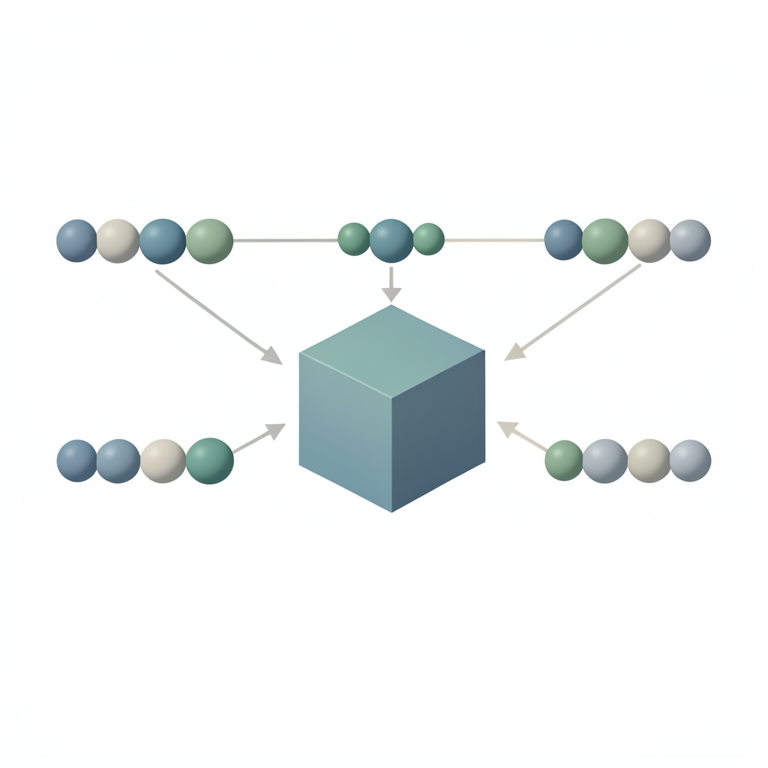
Markov Chain Risk Model ComponentsClose ×

AI-generated conceptual illustration (A conceptual schematic of an insurance capital system). It explains the idea and does not show study data.

Open full-size image ↗

Introduction

Insurance models have been studied by many authors in terms of formulating the ruin probability estimation formula for those models. The second approach is to build a formula for calculating the ruin probability, in Claude Lefèvre and Stéphane Loisel [1], the authors have built a formula of ruin probability for compound biomial and compound Poisson risk models. The result is extended. the formula for calculating the ruin probability of Pircard and Lefèvre [9]. For the general risk model with the impact of interest rates determined by (1.1) below. 1(1 ) ; 1,2,... t t t t t Z Z I X Y t       (1) With Zt is the capital at period t, Zo= z is the capital of the first period of the insurance company; u; t takes the value in the set * {1;2;3;.....} N  ; 1 i i X X   are premiums;  1 j jY Y   are claims and  1 k k I I   are interests.

The approaches of Claude Lefèvre và Stéphane Loisel do not build a formula for calculating the ruin probability. To build the formula for calculating the ruin probability for model (1.1), we assume that the random variable sequences are Markov chains with positive integer values, which is consistent with practice. The article is structured as follows: in Section 2 we introduce model, asumptions; in Section 3, we study the model (1.1) to establish the formula for calculating the ruin probability and the non ruin probability; Finally, in section 4, we introduce the conclusion of this paper. 2. Model and Assumptions To study the model posed for the problem of this paper, we make the following assumptions: Assumption 1. o Z z  , t takes the value in the set * {1;2;3;.....} N  .

Maths 2023; 8(3): 191-198 https://www.mathsjournal.com Phung Duy Quang Foreign Trade University, Hanoi, Vietnam Luu Thi Van Anh University of Transport Technology, Vietnam Bui Duc Duong Luong The Vinh High School, Ha Noi, Vietnam Nguyen Duy Phuong People’s Security Academy, Ha noi, Vietnam Nguyen Van Hoang Foreign Trade University, Hanoi, Vietnam Phung Duy Quang Foreign Trade University, Hanoi, Vietnam https://www.mathsjournal.com Assumption 2. Xn is premium amounts from the nth premium;   1 n n X X   is a Markov chain and is homogeneous, n X take values in   1 2 1 2 , ,..., (0 ... ). X K K T x x x x x x      K Let 1 ,( ); , ij n j n i i j X q P X x X x n N x x T           1 0 1, 1 ij ij j q q            and 1 ( )( ). i i i X q P X x x T    We make the following convention (0 ) 1 n K P X x    , ( 0) 0 if if ( 0) 1 n n P X and P X     . Assumption 3.

Yn is claim amounts from the nth claim,  1 n n Y Y   is a Markov chain and is homogeneous, nY take values in   1 2 1 2 , ,..., (0 ... ). Y P P T y y y y y y      P Let 1 ,( ); , ij m j m i i j Y p P Y y Y y m N y y T           1 0 1, 1 ij ij j q q            and 1 ( )( ). i i i Y p P Y y y T    We make the following convention (1 ) 1 m P P Y y    , ( 0) 0if if ( 0) 1 m m P Y and P Y     . Assumption 4. In is interest amounts from the nth interest,  1 n n I I   is a Markov chain and is homogeneous, nI take values in   1 2 1 2 , ,..., (0 ... ).

I Q Q T i i i i i i      Q Let 1 ,( ); , lh n l n h l h I r P I r I r n N r r T           1 0 1, 1 lh lh h r r            and 1 ( )( ). k k k I r P I r r T    We make the following convention (0 ) 1. n Q P I i    a. X, Y and I are sequences of independent random variables. From (1.1), we have: t t t  1 t k k k j t t k k j k Z z I X Y I X Y 1 1 1 . (1 ) ( ) (1 )                    . (2) The ruin time is defined by   inf : 0 z j T j Z   , where    inf . With assumption 2.1 to assumption 2.5: The finite time ruin probabilities of model (1.1) is defined as: https://www.mathsjournal.com t (3) t z j j z P T t P Z  1 ( ) ( ) ( 0)            The finite time non ruin probabilities of model (1.1) is defined as: t . (4) t t z j j z z P T t P Z 1 ( ) 1 ( ) ( 1) ( 0)              The problem posed in this paper is to build formulas for ( ) t z  and ( ) t z  .

We first prove the following lemma. Lemma 2.1. Assuming z, ( 1, ), ( 1, ) i i x i t y i t   are positive integers và ( 1, ) ki k t  is non - negative number. If n is a possitive integer number that1 1 n t   satisfies: n n n  1 n k k k j n k k j k y z i x y i x             (5) 1 1 1 (1 ) ( ) (1 ) Then   1 1 n n n k k k j n k k j k z i x y i x              (6) 1 1 1 1 (1 ) ( ) (1 ) 1 Proof Use (2.4), we infer n n n  1 y z i x y i x       (1 ) ( ) (1 )    n k k k j n k k j k    1 1 1 n n n  1        x y z i x y i (1 ) ( ) (1 )    n n k k k j k k j k    1 1 1 We have   1 1 n n n k k k j n k k j k z i x y i x             1 1 1 1 (1 ) ( ) (1 ) n n n    1 1 1 = k k k j n n n n k k j k z i x y i x y i x                 1 1 1 1 1 (1 ) ( ) (1 ) ( )(1 ) n n n n n n     1 1 1 1 k k k j k k k j n n k k k j k k j k z i x y i z i x y i i x         1 1 1 1 1 1 1 1 (1 ) ( ) (1 ) (1 ) ( ) (1 ) (1 )                         1 1 nx    .

So (2.5) is correct. Lemma 2.1 has been proved  3. The main result The main result of the paper is that we will build a formula for the ruin probability (2.2) and a formula for the non-ruin probability (2.3). Theorem 3.1.

Consider model (1.1) with Assumption 2.1 to Assumption 2.5, then finite time non ruin probability of model (1.1) is defined by https://www.mathsjournal.com Q K (1) 1 1 2 1 1 1 2 1 1 1 2 1 , ,.., 1 , ,..., 1 1 1 1 ( ) ... ... ... ... t t t t t t            t d d d d d m m m m m n n n n n c c c m m m n f n f n f z r r r q q q p p p  1 2 1 2 1 1 2 2 t t t t            , (7) Where 1 1 1 1 1 1 max : min (1 ) , k n d m P k f n y u i x y                            , 2 2 1 2 2 2 2 1 1 1 ax : min (1 ) ( ) (1 ) , k k k j n d m n d m P k k j k f m n y u i x y i x y                                      , t t t  1 t t n d m m d m P k k j k f m n y u i x y i x y 1 1 1 ax : min (1 ) ( ) (1 ) , t k k k j t                                      , and  a is integer part of a. Proof. Firtly, we let t 1 2 2 1 1 1 2 2 1 1 1 1 (1 ) (1 ) ( ) (1 ) k k k k j k k k j k Y z I X Y z I X Y I X     j j A Z 1 : ( 0)                                3 3 2 t t t  1 3 3 1 1 1 (1 ) ( ) (1 ) ... k k k j k k j k Y z I X Y I X    1 1 1 ... (1 ) ( ) (1 ) t k k k j t k k j k Y z I X Y I X                                    (8) By Asumption 2.4, we have t d d t d I i I i I i    with 1 2 1 2 , ,..., t d d d i i i are non-negative numbers statisfy: 1 2 , ,..., 1 2 0 , ,..., t d d d Q i i i i   . Let       1 2 1 2 ... 1 2 ... t t d d d d d t d B I i I i I i        .

Because  1 n n I I   is a Markov chain and it is homogeneous then      1 2 1 2 ... 1 2 ( ) ... t t d d d d d t d P B P I i I i I i                 1 2 1 1 1 1 2 1 1 2 1 1 . ... ... t t t t d d d t d t d d d d d d P I i P I i I i P I i I i r r r           (9) By Asumption 2.2, we have t m m t m X x X x X x    with 1 2 1 2 , ,..., t m m m x x x are possitive numbers statisfy: 1 2 , ,..., 1 2 0 , ,..., t m m m M x x x x   Define       1 2 1 2 ... 1 2 ... t t m m m m m t m C X x X x X x        . Because   1 n n X X   is a Markov chain and it is homogeneous then      1 2 1 2 ... 1 2 ( ) ... t t m m m m m t m P C P X x X x X x              (10) t t m m m m m p p p 1 1 2 1 ... https://www.mathsjournal.com Firsly, we have 1 1 1 ( 1, ) d I i d Q   then (3.2) is given 1 Q as 2 2 1   1 (1 ) k 1 d d k d A I i Y z i X   1 1 1 1 1 2 2 1 2 1 (1 ) (1 ) ( ) (1 ) d k k k j k k j k Y z i I X Y I X    1                                 3 3 2 t t t  1 1 3 3 1 2 1 (1 ) (1 ) ( ) (1 ) ... d k k k j k k j k Y z i I X Y I X    1 2 1 ... (1 ) (1 ) ( ) (1 ) t d k k k j t k k j k Y z i I X Y I X                     1                    Where as A B  if ( ) 0 P A B   and     \ \ A B A B B A   . Similarly, we let 2 2 2 ,..., ( ,..., 1, ) t d t d t I i I i d d Q    , (3.2) is defined as 1 Q as ... (1 ) t k         1 2 d d t d d k c c c A I i I i I i Y z i X 1 2 1 1 1 , ,..., 1   1 2 t                     2 2 1 3 3 2 2 2 1 1 1 (1 ) ( ) (1 ) k j d k k d k k j k Y z i X Y i X    3 3 1 1 1 (1 ) ( ) (1 ) ... k j d k k d k k j k Y z i X Y i X                                    t t t  1 1 1 1 ... (1 ) ( ) (1 ) k j t d k k d t k k j k Y z i X Y i X                      Next, we let 1 1 1 ( 1, ) m X x m K   , then 1 Q K as 1 2 1 1         1 2 1 1 d d t d m d m k d d d x A I i I i I i X x Y u i x 1 , ,..., 1 1 ... ( ) (1 ) t k    1 2 1 t                           2 2 1 2 2 1 1 1 (1 ) ( ) (1 ) k k j d m k d k k j k Y z i x Y i X                    3 3 2 1 3 1 3 2 1 1 (1 ) ( ) ( ) (1 ) ... k j d m k k d k k j k Y z i x Y X Y i X                            t t t  1 1 1 2 1 1 ... (1 ) ( ) ( ) (1 ) k j t d m k k d t k k j k Y z i x Y X Y i X                                 Similarly, we let 2 2 2 ,..., ( ,..., 1, ) t m t m t X x X x m m K    , (3.2) is defined as Q K as           1 2 d d t d t t d d d m m m A I i I i I i X m X m X m 1 2 1 1 2 2 , ,..., 1 , ,..., 1 ... ( ) ( ) ... ( ) t   1 2 1 2 t t                  1 2 2 1 1 2 1 (1 ) k d m k Y z i x  1 1 1 1 (1 ) ( ) (1 ) k k j d m k d m k k j k Y z i x Y i x                2                 https://www.mathsjournal.com 3 3 2 t t t  1 3 3 1 1 1 (1 ) ( ) (1 ) ... k k j d m k d m k k j k Y z i x Y i x    1 1 1 ... (1 ) ( ) (1 ) k k j t t d m k d m k k j k Y z i x Y i x                                     1 2 1 2 1 2 t t t       1 2 Q K as d d d d d t d m m t m m m m d d d m m m I i I i I i X x X x X x D ... 1 2 1 2 ... , ,.., 1 , ,.., 1 ( ) ( ) ... ( ) ( ) ( ) ... ( ) t   1 2 1 2 t t                        t (11) A B D   1 2 1 2 1 2 1 2 t t t Q K as d d d d d d m m m m m m d d d m m m ... ... ... ... , ,.., 1 , ,.., 1   1 2 1 2 t t            Where 1 2 2 1 ... 1 2 ... 1 2 1 2 1 2 t k k k j as d d d m m m d m d m k d m k k k j k D Y z i x Y z i x Y i x 1 1 1 1 (1 ) (1 ) ( ) (1 ) t                                 3 3 2 t t t  1 3 3 1 1 1 (1 ) ( ) (1 ) ... k k j d m k d m k k j k Y z i x Y i x    1 1 1 ... (1 ) ( ) (1 ) k k j t t d m k d m k k j k Y z i x Y i x                                    (12) By Assumption 2.3, we have 1 2 1 1 2 1 , ,..., ; t n n t n t t Y y Y y Y y Y y       with 1 2 1 , ,..., ; t t y y y y  are positive numbers satisfy: 1 2 0 , ,..., t P y y y y   . Thus, (3.6) is defined as ... 1 2 .... t as d d d m m m ... 1 2 t y z i x y z i x y i x y u i x y i x D (1 ) (1 ) ( ) (1 ) (1 ) ( ) (1 ) 1 2 2 3 3 1 2 1 2 3 1 2 3 1 1 1 1 1 1 1 d m d m n d m d m n d m k k k k j k k k j k k k k j k k j k                                                            Y y Y y (13) 1 n t n                    1 1 (1 ) ( ) (1 ) ... ( ) ... ( ) ... t t t t y z i x y i x t d m n d m k k k j t k k j k    1 1 1                        1 Where, by Lemma 2.1, 1    , (1 ) k d m k z i x  1 2 2 1 t t t 1 1 1 1 (1 ) ( ) (1 ) k k k j d m n d m k k j k z i x y i x            ,…, d m n d m k k j k z i x y i x            are integer 2 1 1 1 (1 ) ( ) (1 ) k k k j numbers and 1 2 0 , ,..., t m m n P y y y y   then, we let 1 1 1 1 1 1 ax : min (1 ) , k n d m P k f m n y z i x y                            , 2 2 1 2 2 2 2 1 1 1 ax : min (1 ) ( ) (1 ) , k k k j n d m n d m P k k j k f m n y z i x y i x y                                      https://www.mathsjournal.com t t t  1 t t t d m n d m P k k j k f m n y z i x y i x y 1 1 1 ax : min (1 ) ( ) (1 ) , k k k j t                                      and  a is integer part of a, Thus, (3.7) is defined as ... 1 2 1 2 t t         1 2 as d d d m m m n n t n n f n f n f D Y y Y y Y y ... 1 2 1 1 1 ... ... t              (14) 1 1 2 2 t t Because  1 n n Y Y   is a Markov chain and it is homogeneous then       1 2 1 1 2 1 1 2 ... ... t t t n n t n n n n n n P Y y Y y Y y q q q             t n n t n Y y Y y Y y       in (3.8) be incompatible then In the other hand, because system of events         1 2 1 2 ... ... 1 2 ... 1 2 1 1 2 1 t t t 1 1 1 ( ) ... ... t          (15) d d d m m m n n n n n n f n f n f P D q q q 1 1 2 2 t t Under the assumption that X, Y and I are sequences of independent random variables then 1 2 ... ... ... ... , , t 1 2 1 2 1 2 t t t d d d d d d m m m m m m B C D are t ... ... ... ... independent events.

Simultaneously, system of events   1 2 t t t d d d d d d m m m m m m B C D   in (2.10) be incompatible. 1 2 1 2 1 2 Therefore, combining (3.3), (3.4) and (3.9), we have. Q K   1 2 1 2 1 2 1 2 t t t d d d t d d d m m m m m m d d d m m m z P A P B C D  ... ... ... ... , ,.., 1 , ,..., 1 ( ) ( ) t   1 2 1 2 t t             Q K P B P C P D . . t =       1 2 1 2 1 2 1 2 t t t d d d d d d m m m m m m d d d m m m ... ... ... ... , ,..., 1 , ,..., 1   1 2 1 2 t t         Q K 1 1 2 1 1 1 2 1 1 1 2 1 d d d d d m m m m m n n n n n d d d m m m n f n f n f r r r p p p q q q            1 2 1 2 1 1 2 2 , ,.., 1 , ,..., 1 1 1 1 ... ... ... ... t t t t t t t t t t            (15) Theorem 3.1. Has been proved. Corollary 3.1.

Consider model (1.1) with assumption 2.1 to assumption 2.5, then finite time ruin probability of model (1.1) is defined as ( ) 1 ( ) t t z z    Q K 1 1 2 1 1 1 2 1 1 1 2 1 d d d d d m m m m m n n n n n d d d m m m n f n f n f r r r p p p q q q            1 2 1 2 1 1 2 2 , ,.., 1 , ,..., 1 1 1 1 1 ... ... ... ... t t t t t t t t t t            (16) Remark 3.1. Formula (3.11) allows to calculate the ruin probability of the model (1.1) assuming that the series of insurance premium, the series of insurance claim, and the series of interest rates are sequences of random variables that depend on Markov and receive the value positive integers. Formula (3.1) allows to calculate the non-ruin probability of the model (1.1) assuming that the series of insurance premium, the series of insurance claim, the series of interest rates are sequences of random variables that depend on Markov and receive the value positive integers. https://www.mathsjournal.com

Conclusion

Using the tools of probability theory, we have built a formula to calculate the ruin probability (The non-ruin probability) of a general insurance model with a series of Markov dependent random variables and receive the following values: positive integers. Our main result in this paper is Theorem 3.1.

1. Lefèvre C, Loisel S. On finite - time ruin probabilities for classical models, Scandinavian Actuarial Journal. 2008;2008(1):56-68.
2. De Vylder FE. La formule de Picard dt Lefèvre pour la probabilité de ruine en temps fini, Bulletin Francais d’Actuariat. 1997;1(2):31-40.
3. De Vylder FE. Numerical finite – time ruin probabilities by the Picard – Lefèvre formula. Scandinavian Actual Journal. 1999;1999(2):97-105.
4. De Vylder FE, Goovaerts MJ. Recursive calculation of finite-time ruin probabilities, Insurance: Mathematics and Economics. 1998;7(1):1-7.
5. De Vylder FE, Goovaerts MJ. Explicit finite – time and infinite – time ruin probabilities in the continuous case. Insurance: Mathematics and Economics. 1999;24(3):155- 172.
6. Gerber HU. An Introduction to Mathematical Risk Theory. Insurance: Mathematics and Economics. 1979;24:155-172.
7. Ignatov ZG, Kaishev VK, Krachunov RS. An improved finite – time ruin probability formula and its Mathematical implemention. Insurance: Mathematics and Economics. 2001;29(3):375-386.
8. Ignatov ZG, Kaishev VK. A finite – time ruin probability formula for continuous claim severities. Journal of Applied Probability. 2004;41(2):570-578.
9. Picard PH, Lefèvre CL. The probability of ruin in finite time with discrete claim size distribution. Scandinavian Actuarial. 1997;1997(1):58-69.
10. Quang PD. Upper Bounds for Ruin Probability in Generalized Risk Processes under rates of interest with homogenous Markov chain claims and homogenous Markov chain premiums, Applied Mathematical Sciences. 2014;8(29):1445-1454.
11. Quang PD. Ruin Probability in a Generalised Risk Process under Rates of Interest with Homogenous Markov Chains, East Asian Journal on Applied Mathematics. 2014;4(3):283-300.
12. Quang PD, Chien DQ, Thinh NH. Simulation for Ruin Probabilities in Insurance with Sequence Markov Dependence Random Variables, Universal Journal of Accounting and Finance. 2021;9(5):927-934.
13. Rullière D, Loisel ST. Another look at the Picard – Lefèvre formula for finite – time ruin probabilities. Insurance: Mathematics and Economics. 2004;35(2):187- 203.