
Research article · 2023 · Full text
International Journal of Statistics and Applied MathematicsPotato yield forecast models for Sultanpur district of eastern Uttar Pradesh using discriminant function analysis
Volume 8(2) · Pages 39–42 · DOI: 10.22271/maths.2023.v8.i2a.943 ↗
Research areasAgricultural Economics and Practices
Abstract
Author-writtenThe development of the pre-harvest forecast model has made use of time series data on potato yield as well as weekly data on five weather variables, including Minimum Temperature, Maximum Temperature, Relative Humidity 08.30 hrs, Relative Humidity 17.30 hrs, and Wind-Velocity, for the period from 1990-91 to 2011-2012. For the development of a pre-harvest forecast model, statistical approaches utilising discriminant functions analysis have been described. Six models have been created altogether using discriminant functions analysis. The two best models produced by using weekly weather data are Model- II and Model- Vth, based on adjR2, RMSE percent deviation, and % SE. Two and a half months prior to harvest, these models can be utilised to obtain a trustworthy forecast of potato productivity.
Summary
Source-checkedPlain-language reading of the full paper, prepared with AI and checked against the text. Each point links to the authors' own words.
Why it matters
- Weather significantly influences crop growth by directly affecting structural parameters and indirectly impacting the occurrence of pests and diseases. View evidence ↗
- Analyzing weather factors during different growth stages can help predict final crop yields before the harvest occurs. View evidence ↗
The question
- The study aims to develop potato yield forecast models using weather data and discriminant function analysis. View evidence ↗
What they did
- The researchers used 22 years of potato yield time series data (1990-91 to 2011-2012) from the Sultanpur district of Uttar Pradesh. View evidence ↗
- Yield modeling was performed using data from 1991 to 2008 (18 years), while data from 2009 and 2010 were used for validation. View evidence ↗
- The statistical models were built using 19 weeks of meteorological data, spanning from the 40th standard meteorological week (SMW) of one year to the 6th SMW of the next. View evidence ↗
- Six distinct procedures were employed to create six different forecast models. View evidence ↗
What they found
- Model-II demonstrated a coefficient of determination (R2) of 65.92% and the lowest Root Mean Square Error (RMSE) of 3.55. View evidence ↗
- Model-V was identified as the second-best model based on its RMSE, percent deviation, and percent standard error. View evidence ↗
- Overall, Model-II and Model-V were found to be the most appropriate for forecasting potato yields in the Sultanpur district. View evidence ↗
What it means
- The authors conclude that Model-II and Model-V can accurately predict potato yields approximately two and a half months before harvest. View evidence ↗
Visual summary
2 visualsIllustrations explain the paper; charts are replotted from the paper's own table values.
Potato Yield Forecasting Workflow
AI-generated conceptual illustration (Potato plants in a field). It explains the idea and does not show study data.
View source evidence ↗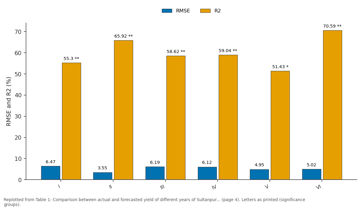
RMSE and R2: I vs II vs III vs IV vs V
Replotted from Table 1 (page 4) of the original paper. Every bar is the paper's own table value.
View source evidence ↗Figures & tables
From the original paper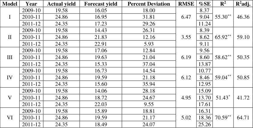 Table 1
Introduction
The most significant vegetable crop in India is the potato, also referred to as "the king of vegetables" (Solanum tuberosum L.). The most significant cash crop in Uttar Pradesh is it. It yields more dry matter, edible energy, and edible protein in a shorter amount of time than cereals like rice and wheat since it is a short-duration crop. It is a South American tropical native. In the 2012-13 growing season, India produced roughly 453.44 lakh tonnes of potatoes on 19.92 lakh hectares. The states of Uttar Pradesh, West Bengal, Bihar, and Punjab contributed the majority of the produce in 2012-2013, with contributions of 32, 26, 15, and 5%, respectively. The most significant vegetable crop in India is the potato, also referred to as "the king of vegetables" (Solanum tuberosum L.). The most significant cash crop in Uttar Pradesh is it. It yields more dry matter, edible energy, and edible protein in a shorter amount of time than cereals like rice and wheat since it is a short-duration crop. It is a South American tropical native. In the 2012-13 growing season, India produced roughly 453.44 lakh tonnes of potatoes on 19.92 lakh hectares. The states of Uttar Pradesh, West Bengal, Bihar, and Punjab contributed the majority of the produce in 2012-2013, with contributions of 32, 26, 15, and 5%, respectively. A composite model can be produced by using any one of these methods alone or in combination. One of the key elements affecting crop growth is the weather. It may have a direct impact on crop growth structural parameters including plant population, number of tillers, leaf area, etc., as well as a secondary impact on pest and disease incidence. The influence of weather factors at various phases of crop growth may aid in understanding how the crop will respond in terms of final yield and can offer a forecast of crop yields before harvest. The quantity of meteorological characteristics and their frequency distribution alone determine how much the weather affects agricultural production. Hence, in creating the preharvest model, understanding the frequency distribution of weather parameters is very crucial. The relationship between crop weather and crop production prediction has been the subject of numerous research in the past, both in India and overseas. The first attempt to establish a cropweather link was undertaken by Fisher (1924) [1] . The Fisher's technique was updated by Hendrics and Scholl in 1943 [2] .
The method of Hendrics and Scholl (1943) [2] was further refined by Agarwal et al. (1980) [3] by creating a forecast model employing meteorological indices for the rice crop in the Chhattisgarh district of Raipur. Many authors have used this method of Agarwal et al (1980) [3] in the past to develop predicted yields of various crops in various regions of the nation. Discriminant function analysis has been used by Agrawal et al. (2012) [6] , Sisodia et al. (2014) [7] , Azfar et al. (2014), Azfar et al. (2015) [1] , and Yadav et al. (2016) [12] to create forecast models for specific crops. The goal of the current study is to use discriminant function analysis to create forecast models for potato yield based on weather data.
Materials and Methods
This is a presentation of the resources used and the methods used to create forecast models.
Description of the Study Area
The coordinates of Sultanpur are 26.27° N 82.07° E. It covers 1,713 square miles (4,437 km2). Only the ravines near the rivers, which normally have a level surface, cause this. While the southern region is largely made up of marshes and barren plains, the centre region is heavily farmed. The Gomti river, which flows through the district's heart, is the main river. 3,790,922 people made up the Sultanpur district as per the 2011 Census. As a result, it is ranked 69th in India (out of a total of 640). There are 855 people living there per square kilometer, or 2,210 per square mile. Its population grew at a 17.92% annual pace between 2001 and 2011. Sultanpur has a 978 girls to 1000 males sex ratio and a 71.14% literacy rate.
Yield data
From the Bulletins of the Directorate of Agricultural Statistics and Crop Insurance, Government of Uttar Pradesh, time series data on potato yield in Sultanpur district of Uttar Pradesh over 22 years (1990-91 to 2011-2012) have been gathered.
Weather data
Monthly meteorological data for the same period on five weather variables viz., Minimum Temperature, Maximum Temperature, Relative Humidity at 8.30 and 17.30 hrs and Wind-Velocity have been employed in the study. The Department of Meteorological Center at Amausi Airport in Lucknow provided the weekly data on these weather factors. India's U.P.
Statistical Tools Used in the Analysis
The following statistical tools and methodologies have been applied while keeping in mind the goals of the investigation. SPSS and MS-EXCEL are two examples of the software used to analyse the data.
Statistical methodology
The method of discriminant function analysis offers a suitable function that distinguishes between two or more groups and categorises the upcoming data into one of the previously established groups. Assume that p variables are used to divide observations into k non-overlapping groups. The method locates linear functions where the coefficients of the variables are chosen so that the variance within the groups is minimised and the variation between the groups is maximised. The least of (k-1) and p determines the smallest number of discriminant functions that can be obtained. Discriminant scores, which are used to divide the observations into various groups, are computed using these functions.
In the Kanpur area of Uttar Pradesh, Agrawal et al. (2012) [6] were the first to construct prediction models for wheat production using the discriminant function analysis technique, which offered a reliable yield forecast around two months before harvest. In order to create adequate models for preharvest forecast of potato yield in Sultanpur district of Uttar Pradesh, this paper uses their method with a few modifications. Crop years have been divided into congenial, normal, and adverse groups based on crop yield adjusted for trend effect in order to apply discriminant function analysis for modelling yield using weather variables. These three groups' meteorological data were utilised to create linear discriminant functions, and each year's discriminant scores were calculated. The forecast models were created using these scores, the year as a regressor, and crop yield as a regress and. Since there are three groups and five meteorological variables in the current study, only two discriminant functions are necessary to classify a crop year into one of the three categories. These are the three groups of crop years, namely unfavourable, normal, and congenial: Let y and s represent the average and range of agricultural production after adjusting for n years. Adjusted crop yields less or equal to y-s would be in the unfavourable group, those between y-s and y+s would be in the normal group, and those above or equal to y+s would be in the congenial group. Yet, it is well known that the crop is affected by meteorological variables differently depending on the stage of crop development. Its impact is influenced by both its size and how it is dispersed over the growing season. Since there would be an enormous increase in the number of independent variables in the regression model, using weekly meteorological data as such to create the model presents a challenge. The following weather indices have been created using the Agrawal et al. approach to address this issue (1980) [3] . Where Zij is un-weighted (for j=0) and weighted (for j=1) weather indices for ith weather variable and is the unweighted (for j=0) and weighted (for j=1) weather indices for interaction between ith and i'th weather variables. Xiw is the value of the ith weather variable in the corresponding week, riw/rii'w is the yield correlation coefficient adjusted for trend effect with the ith weather variable/product of the ith and i'th weather variables in the corresponding week, n is the number of weeks taken into consideration in developing the indices, and p is the number of weather variables. Here, p=5 and n=15, or data from 15 weeks from the 44th to the 52nd week of a year and the first to the sixth week of the following year, have been used to create weighted and unweighted weather indices of weather variables as well as their interactions. All told, 30 indices-15 weighted and 15 unweighted-have been created, with the composition being 5 weighted weather indices, 10 weighted interaction indices, 5 unweighted and 10 unweighted interaction indices. Moreover, some better tactics have been proposed. Six potential models are explored in total. The first two are the top models identified by Agrawal et al. (2012) [6] , whereas the latter four are brand-new ideas. Regression analysis is used in the creation of models. Only the first 18 years' worth of data, from 1991 to 2008, were used to model yield, and the final two years' worth of data, from 2009 and 2010, were used to validate the models.
Development of forecast model using discriminant Function Analysis
Procedure-1 This makes use of all of the data from the 19 weeks, as well as the relative weight of meteorological variables for each week. Two discriminant functions were produced after conducting a discriminant function analysis using five weighted weather indices of five different weather variables as the discriminating factors. Using these two discriminant functions, two sets of discriminant scores for the years under consideration were derived. These two sets of discriminant scores, coupled with the trend variable and the yield as the regress and, were used to produce the forecast. Following is the form of consideration:
where y = crop yield, 0 β = intercept, βi's (i =1,2,3)= the regression coefficients ds1 and ds2 are the two discriminant scores, T is the trend variable and
Procedure-2
This is 4 th of Agrawal et al. (2012) [6] . Two discriminant functions and there from two sets of discriminant scores have been obtained using the first week data (40 th SMW) on five weather variables. Next, two sets of discriminant scores obtained from first week data and second week (41 th SMW) data on five weather variables have been used as discriminating variables. So in all there were 7 discriminating variables and based on these 7 discriminating variables, the discriminant function analysis has been done and therefore, two sets of discriminant scores have been obtained. Until the forecast (6th SMW or 19th week), this process is repeated, at which point two sets of discriminant scores have been obtained. The forecasting using yield as the regress and, the discriminant scores, and the trend variable (T) as the regressor variables has been fitted based on these two sets of discriminant scores. This model's structure is comparable to the model presented in equation no (2).
Procedure-3
Five weighted and five unweighted weather indices were employed as discriminating variables in this model. Now that the discriminant function analysis has been completed using these 10 indices, two sets of scores have been acquired. The yield has been used as the regressand in the regression that has been fitted using these two sets of scores as the dependent variable, along with the two sets of scores and the trend variable (T). This model's structure is comparable to the model presented in equation no (2).
Procedure-4
Two sets of discriminant scores from two discriminant functions have been generated in this study using all 30 indices (weighted and unweighted, including interaction indices) as discriminating factors in the analysis of the discriminant function. Using the untrended yield as the regressand variable, the two sets of discriminant scores, and the trend variable (T) as the regressor variables, forecasting has been fitted. This model's structure is similar to how equation ( 2) has been fitted.
Procedure-5
This discriminant function analysis was done using weekly data from the first weather variable distributed over a period of 19 weeks. The discriminant function analysis has been repeated using two sets of discriminant scores from two estimated discriminant functions based on data from the first weather variable and 19 weeks' worth of data from the second variable (here the discriminating variables will now become 21). Following the completion of discriminant analysis using these two sets of discriminant scores and 19 weeks' worth of data for the third weather variable, two sets of discriminant scores have been acquired. Two sets of discriminant scores, ds1 and ds2, were obtained after this process was continued up to five meteorological variables. These two sets of scores are used to create a forecast by fitting a model identical to the one in equation no., with the trend variable (T) serving as the regressor variable and crop yield as the regressand (2).
Procedure-6
The first weather variable's unweighted and weighted averages (weather indices) have been used in this discriminant function analysis (here discriminating factors will be only two). Discriminant function analysis has been further performed using the two sets of discriminant scores obtained on the basis of the first weather variable and un-weighted and weighted averages (weather indices) for the second weather variable (here, the discriminating factors will be four). We carried on with this process until the fifth weather variable, at which point we obtained the ds1 and ds2 sets of discriminant scores. Crop yield is used as the regressand, and the discriminant scores ds1 and ds2 as well as the time trend variable (T) are used as the regressor to fit a model similar to the one in equation no (2).
Results and Discussion
On the basis of the methods outlined in the preceding section, numerous pre-harvest forecast models have been created. The following is a presentation of the findings, outcomes, and pertinent debate.
Forecast Model-I: Y = 14.605 + 1.469ds1 -1.120ds2 + 0.063T Forecast Model-II Y = 15.85 + 0.01ds1 + 0.31ds2 -0.01T Forecast Model-III Y = 15.296 + 1.828ds1 -1.522ds2 + 0.10T Forecast Model-IV Y =15.556+ 1.840ds1 + 1.484ds2 -0.014T Forecast Model-V Y = 15.914 -0.786ds1 -0.731ds2 + 0.033T Forecast Model-VI Y = 15.214 -1.467ds1 -1.165ds2 + 0.024T Six different procedures were used to construct each of the six models. In Sultanpur district, potato sowing typically begins in the first week of October. As a result, weekly weather data have been taken into account starting with the 40th SMW of crop, which falls during the first week of October. Pre-harvest forecasting of the potato production has been suggested to be done during the milking or dough stage, or roughly two months before the harvest. Generally speaking, the milking and dough periods begin 130 days or so following seeding. Thus, the sixth SMW of the following year (February 5-February 11) has been designated as the pre-harvest forecast week. This means that a total of 19 weeks' worth of meteorological data-from the 40th SMW of one year ago to the 6 th SMW of the following year-have been used to build the statistical models. Based on the aforementioned six steps, all six models were created. The models found are provided below.
Comparison of the model
The forecast yields for the 2009-10, 2010-11, and 2011-12 have been calculated based on these six forecast models, and the results are shown in Table 1. For each model, the values of R2adj, RMSE, and % SE (CV), as well as the percent deviation of forecast from actual yield, have also been computed and are also shown below. The results of Table 1 clearly show that the Model-coefficient II's of determination (R2) was determined to be 65.92% with a lower percentage standard error and a minimal RMSE of 3.55. Model-V, which is based on RMSE, percent deviation, and percent SE, comes next. The Model-II and Model-V are the most appropriate models among all the models to forecast potato yield in the Sultanpur district of Eastern Uttar Pradesh, according to the overall results of Table 1. As a result, both the Model-II and Model-V can provide an accurate prediction of potato yield roughly two and a half months prior to harvest.
| Model | Year | Actual yield | Forecast yield | Percent Deviation | RMSE | %SE | R2 | R2adj. |
|---|---|---|---|---|---|---|---|---|
| I | 2009-10 | 19.58 | 16.05 | 18.00 | 6.47 | 8.37 | 55.30** | 46.36 |
| 2010-11 | 24.86 | 16.95 | 31.81 | 9.04 | ||||
| 2011-12 | 24.35 | 17.23 | 29.26 | 11.24 | ||||
| II | 2009-10 | 19.58 | 14.43 | 26.31 | 3.55 | 8.39 | 65.92** | 59.10 |
| 2010-11 | 24.86 | 21.83 | 12.16 | 8.62 | ||||
| 2011-12 | 24.35 | 22.91 | 5.93 | 9.11 | ||||
| III | 2009-10 | 19.58 | 17.06 | 12.84 | 6.19 | 9.56 | 58.62** | 50.35 |
| 2010-11 | 24.86 | 19.63 | 21.04 | 8.60 | ||||
| 2011-12 | 24.35 | 15.33 | 37.04 | 13.87 | ||||
| IV | 2009-10 | 19.58 | 16.73 | 14.54 | 6.12 | 10.77 | 59.04** | 50.85 |
| 2010-11 | 24.86 | 19.59 | 21.18 | 8.46 | ||||
| 2011-12 | 24.35 | 15.60 | 35.94 | 12.95 | ||||
| V | 2009-10 | 19.58 | 14.06 | 28.18 | 4.95 | 15.09 | 51.43* | 41.72 |
| 2010-11 | 24.86 | 18.72 | 24.67 | 13.70 | ||||
| 2011-12 | 24.35 | 22.03 | 9.55 | 17.61 | ||||
| VI | 2009-10 | 19.58 | 15.89 | 18.81 | 5.02 | 16.31 | 70.59** | 64.71 |
| 2010-11 | 24.86 | 19.59 | 21.17 | 18.36 | ||||
| 2011-12 | 24.35 | 18.49 | 24.07 | 25.26 |
Table text extracted from the original PDF; superscript letters are shown inline. The original table image is below.
View original table image
Summary and Conclusion
Using weekly data on five meteorological factors, discriminant function analysis technique has been used to construct a forecast model for potato yield in the Sultanpur area of Uttar Pradesh. All six models have been created. Based on the parameters of RMSE, percent deviation, and percent SE incorporating coefficient of determination, the models II and V have been determined to be the best among all. These two models can produce accurate forecasts of potato production roughly two and a half months before the harvest.
References
10 in the original paper- Fisher RA. The influences of rainfall on the yield of wheat at Rothamsted. Philosophical Transaction of Royal Society of London, Series B. 1924;213:89-142.
- Hendricks WA, Scholl GC. Technique in measuring joint relationship: The joint effects of temperature and precipitation on crop yield. N. Carolina Agricultural Experiment Station Technical Bulletin, 1943;74:1-34.
- Agrawal, Ranjana, Jain Re, Singh D. Forecasting of rice yield using climatic variables. Indian Journal of Agricultural Sciences. 1980;50(9):680-684.
- Agrawal R, Chandrahas, Aditya Kaustav. Use of discriminant function analysis for forecasting crop yield, Mausam. 2012;63(3):455-458.
- Sisodia BVS, Sunil Kumar, Yadav RR, Sharma MK. Forecasting of Pre-harvest crop yield using discriminant function analysis of meteorological parameters, Journal of Agro-Meteorology. 2014;16(1):121-125.
- Pandey KK, Rai VN, Sisodia BVS. Weather variable based rice yield forecasting modles for Faizabad district of eastern U.P. International Journal of Agricultural and Statistical Sciences. 2014;10(2):381-385
- Mohd. Azfar, Sisodia BVS, Rai VN, Monika Devi. Pre harvest forecast of rapeseed & mustard yield based on weather variables: An application of discriminant function analysis. International Journal of Agricultural and Statistical Sciences. 2014;10(2):497-502.
- Azfar, Sisodia BVS, Rai VN, Sunil Kumar. A study on Impact of Changes in Climate variables on Rice Production. In Faizabad district of Uttar Pradesh. Mausam. 2015;66(2):281-286.
- Yadav RR, Sisodia BVS, Sunil Kumar. Pre-harvest forecast of pigeon-pea yield using discriminant function analysis of weather variables. Mausam. 2016;67(3):577582.
- Snehdeep BVS, Sisodia, Rai VN. Yield Forecast Models of Potato Using Discriminant Function Analysis for Barabanki District of Uttar Pradesh. Frontiers in Crop Improvement. 2021;9(4):2529-2533.