
Research article · 2023 · Full text
International Journal of Statistics and Applied MathematicsConstruction and selection of conditional double sampling plan indexed through AOQcc
Volume 8(1) · Pages 30–35 · DOI: 10.22271/maths.2023.v8.i1a.926 ↗
Research areasAdvanced Statistical Process MonitoringFault Detection and Control SystemsIndustrial Vision Systems and Defect Detection
Abstract
Author-writtenIn this paper a procedure for constructing a Conditional Double Sampling Plan indexed through a parameter which is a convex combination of AOQL (Average Outgoing Quality Limit) and MAAOQ (Maximum Allowable Average Outgoing Quality) with gain parameter λ is given. This plan may safeguard the interests of both producer as well as consumer by properly choosing a right combination using the gain parameter λ. Tables are also constructed for the easy selection of the plan.
Summary
Source-checkedPlain-language reading of the full paper, prepared with AI and checked against the text. Each point links to the authors' own words.
Why it matters
- Conditional double sampling differs from standard double sampling because any necessary second sample is drawn from a related lot rather than the current one. View evidence ↗
- The primary benefit of conditional double sampling is the reduction in sample size while maintaining effective operating characteristic (OC) curves. View evidence ↗
- The Average Outgoing Quality Limit (AOQL) represents the worst average quality a consumer will receive after defective items are replaced. View evidence ↗
The question
- The study aims to provide a procedure for constructing a Conditional Double Sampling Plan (CDSP) indexed through AOQcc to protect both producer and consumer interests using a gain parameter λ. View evidence ↗
What they did
- The proposed plan is indexed through AOQcc, which is defined as a convex combination of the Average Outgoing Quality Limit (AOQL) and the Maximum Allowable Average Outgoing Quality (MAAOQ). View evidence ↗
- The operating procedure involves taking an initial sample (n1); the lot is accepted if non-conformities (d1) are ≤ c1, rejected if d1 > c3, or a second sample (n2) is taken if d1 is between c1+1 and c3. View evidence ↗
What they found
- When indexed by MAAOQ = 0.0023 and MAPD = 0.0037, the sample size is reduced to n1=n2=827 with c1=2, c2=4, and c3=6. View evidence ↗
- Using a compromise gain parameter λ=0.7 (AOQcc=0.00244) with the same quality levels results in a sample size of n1=n2=1686 and parameters c1=5, c2=9, c3=12. View evidence ↗
- At a gain parameter of λ=0.6, the sample size can be as low as 393 for an AOQcc of 0.00242. View evidence ↗
What it means
- The authors conclude that CDSP plans indexed through (MAPD, AOQcc) require smaller sample sizes than those indexed through (MAPD, AOQL). View evidence ↗
- The authors state that these plans effectively protect the interests of both the producer and the consumer. View evidence ↗
Visual summary
1 visualsIllustrations explain the paper; charts are replotted from the paper's own table values.
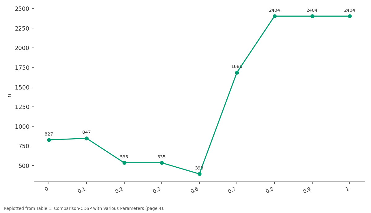
n: 0 vs 0.1 vs 0.2 vs 0.3 vs 0.6
Replotted from Table 1 (page 4) of the original paper. Every bar is the paper's own table value.
View source evidence ↗Figures & tables
From the original paper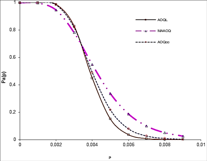 Figure 1
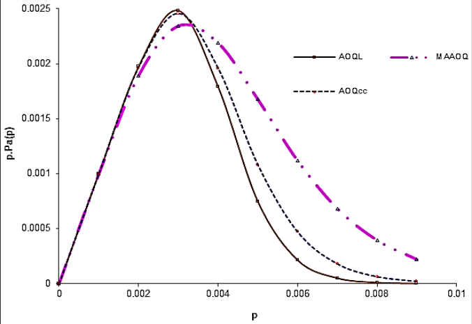 Figure 2
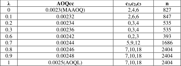 Table 1
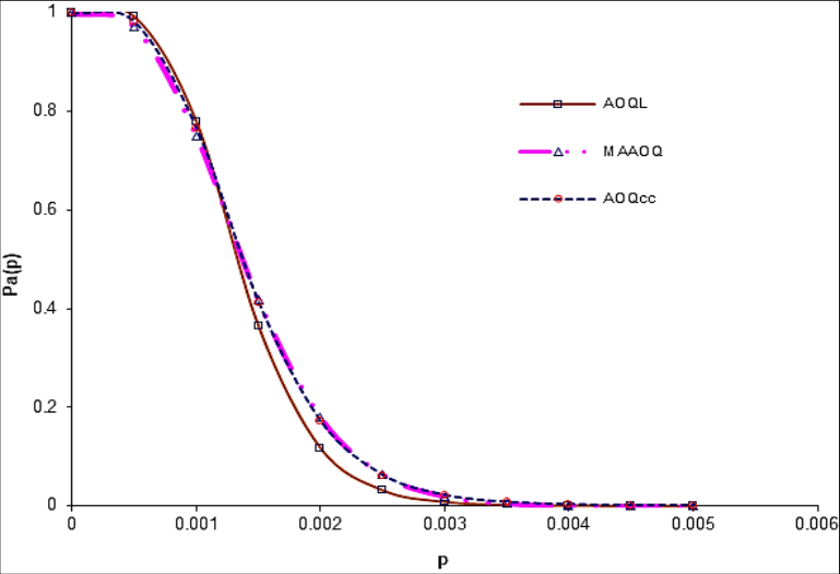 Figure 3
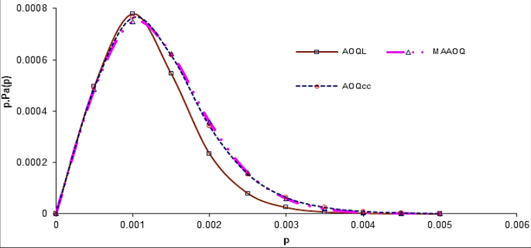 Figure 4
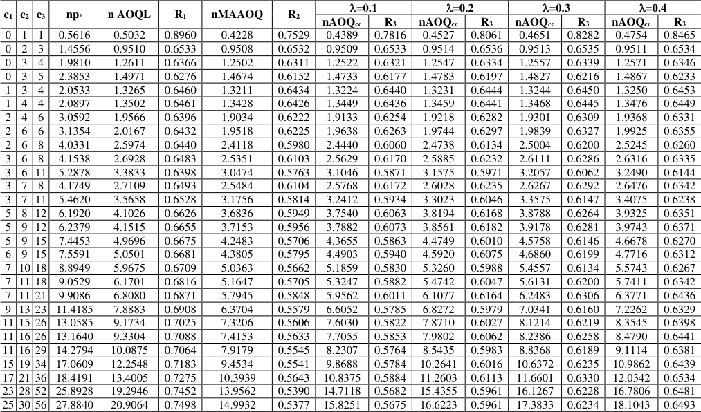 Table 2
Introduction
Conditional sampling plans are called special purpose plans. Baker and Brobst (1978) [1] proposed conditional sampling procedures which are similar to double sampling and these conditional double sampling procedures have Operating Characteristics curves identical to those of comparable double sampling procedures. Conditional double sampling is operationally different form double sampling in that the results of the second sample, if required, are obtained from related lot and not from the current lot. According to Baker and Brobst using sample information from related lots results in more attractive OC curves with smaller sample sizes. This reduction in sample size is the principal advantage of these procedures In this paper a procedure is given to construct Conditional Double Sampling Plan (CDSP) indexed through AOQ cc which safeguards the interest of both producer and consumer by properly choosing the right combination of gain parameter (0<<1). Necessary tables for the selection of the sampling plans are provided.
Definitions 2.1 Definition of AOQL
The AOQL is defined as the worst average that the consumer will receive in the end, when defective items are replaced by non-defective items. It is obtained by maximizing Average Outgoing Quality (AOQ), AOQ= p.P a (p).
Definition of MAPD
The MAPD is the value of fraction defective (p=p*) at which d 2 P a (p)/dp 2 = 0 and d 3 P a (p)/dp 3 ≠ 0 It is also the inflection point of the operating characteristic (OC) curve and Pa(p) is the probability of acceptance at the quality level p fraction defective
Definition of MAAOQ
The MAAOQ is defined as average outgoing quality at MAPD, we have MAAOQ = AOQ at p= p*
Review of Literature
The desirability of developing a set of sampling plans indexed through p*(MAPD) has been explained by Mandelson (1962) [2] and Soundararajan (1975) [7] . Vijayaraghavan (1990) [9] has provided procedures and tables for the selection of conditional double sampling plans for various entry parameters. Suresh and Ramkumar (1996) [8] suggested a procedure for constructing the sampling plans indexed through Maximum Allowable Average Outgoing Quality (MAAOQ).Taking into the criticisms leveled on AOQL by several authors and the importance of MAPD as a quality measure, Radhakrishnan (2002) [3] constructed continuous sampling plan, chain sampling, double and link sampling plan indexed through MAAOQ and established that the size of the sample is less in the sampling inspection when MAAOQ is used as an index parameter than AOQL Sampathkumar (2007) [6] constructed mixed sampling plan with conditional double sampling plan as a reference plan using various entry parameters. Radhakrishnan and Mallika (2008, 2009) [4] constructed Single Sampling Plan indexed through AOQ cc which is the convex combination of AOQL and MAAOQ.
Operating procedure of CDSP
The Operating procedure of CDSP is as follows:
Step 1: Select a random sample of size n (=n 1 =n 2 ) from a lot of size N.
Step 2: Inspect all the articles included in the sample. Let d 1 be the number of non-conformities in the sample.
Step 3: If d 1 ≤c 1 , accept the lot, if d 1 >c 3 , reject the lot.
Step 4: If c 1 +1<d 1 ≤c 3 take a second sample of size n 2 from the remaining lot and find the number of non-conformities d 2 .
Step 5: If d 2 ≤c 2 or d 1 +d 2 ≤c 3 accept the lot, otherwise reject the lot.
Operating Characteristic function
Under the Poisson model, the OC function of the CDSP is given by
Construction and selection of CDSP indexed through AOQcc
The procedure presented in the section 4 is used for designing Conditional Double Sampling Plan indexed through AOQ cc and are presented in Table 2. The values of np * , nMAAOQ, nAOQL and nAOQ cc for the different values of (from 0.1 to 0.9) are calculated using Visual Basic program. Table 2 is used to construct the plan when the np * and nAOQ cc are specified. One can find the ratio R 3 = nAOQ cc /np * and locate the value obtained under the column R 3 (for various values of ) the corresponding value of np * is noted and hence the parameters n 1 , n 2 , c 1 , c 2 , c 3 for CDSP are determined.
| c1 | c2 | c3 | np* | n AOQL | R1 | nMAAOQ | R2 | =0.1 | — | =0.2 | — | =0.3 | — | =0.4 | — |
|---|---|---|---|---|---|---|---|---|---|---|---|---|---|---|---|
| nAOQcc | R3 | nAOQcc | R3 | nAOQcc | R3 | nAOQcc | R3 | ||||||||
| 0 | 1 | 1 | 0.5616 | 0.5032 | 0.8960 | 0.4228 | 0.7529 | 0.4389 | 0.7816 | 0.4527 | 0.8061 | 0.4651 | 0.8282 | 0.4754 | 0.8465 |
| 0 | 2 | 3 | 1.4556 | 0.9510 | 0.6533 | 0.9508 | 0.6532 | 0.9509 | 0.6533 | 0.9514 | 0.6536 | 0.9513 | 0.6535 | 0.9511 | 0.6534 |
| 0 | 3 | 4 | 1.9810 | 1.2611 | 0.6366 | 1.2502 | 0.6311 | 1.2522 | 0.6321 | 1.2547 | 0.6334 | 1.2557 | 0.6339 | 1.2571 | 0.6346 |
| 0 | 3 | 5 | 2.3853 | 1.4971 | 0.6276 | 1.4674 | 0.6152 | 1.4733 | 0.6177 | 1.4783 | 0.6197 | 1.4827 | 0.6216 | 1.4867 | 0.6233 |
| 1 | 3 | 4 | 2.0533 | 1.3265 | 0.6460 | 1.3211 | 0.6434 | 1.3224 | 0.6440 | 1.3231 | 0.6444 | 1.3244 | 0.6450 | 1.3250 | 0.6453 |
| 1 | 4 | 4 | 2.0897 | 1.3502 | 0.6461 | 1.3428 | 0.6426 | 1.3449 | 0.6436 | 1.3459 | 0.6441 | 1.3468 | 0.6445 | 1.3476 | 0.6449 |
| 2 | 4 | 6 | 3.0592 | 1.9566 | 0.6396 | 1.9034 | 0.6222 | 1.9133 | 0.6254 | 1.9218 | 0.6282 | 1.9301 | 0.6309 | 1.9368 | 0.6331 |
| 2 | 6 | 6 | 3.1354 | 2.0167 | 0.6432 | 1.9518 | 0.6225 | 1.9638 | 0.6263 | 1.9744 | 0.6297 | 1.9839 | 0.6327 | 1.9925 | 0.6355 |
| 2 | 6 | 8 | 4.0331 | 2.5974 | 0.6440 | 2.4118 | 0.5980 | 2.4440 | 0.6060 | 2.4738 | 0.6134 | 2.5004 | 0.6200 | 2.5245 | 0.6260 |
| 3 | 6 | 8 | 4.1538 | 2.6928 | 0.6483 | 2.5351 | 0.6103 | 2.5629 | 0.6170 | 2.5885 | 0.6232 | 2.6111 | 0.6286 | 2.6316 | 0.6335 |
| 3 | 6 | 11 | 5.2878 | 3.3833 | 0.6398 | 3.0474 | 0.5763 | 3.1046 | 0.5871 | 3.1575 | 0.5971 | 3.2057 | 0.6062 | 3.2490 | 0.6144 |
| 3 | 7 | 8 | 4.1749 | 2.7109 | 0.6493 | 2.5484 | 0.6104 | 2.5768 | 0.6172 | 2.6028 | 0.6235 | 2.6267 | 0.6292 | 2.6476 | 0.6342 |
| 3 | 7 | 11 | 5.4620 | 3.5658 | 0.6528 | 3.1756 | 0.5814 | 3.2412 | 0.5934 | 3.3023 | 0.6046 | 3.3575 | 0.6147 | 3.4075 | 0.6238 |
| 5 | 8 | 12 | 6.1920 | 4.1026 | 0.6626 | 3.6836 | 0.5949 | 3.7540 | 0.6063 | 3.8194 | 0.6168 | 3.8788 | 0.6264 | 3.9325 | 0.6351 |
| 5 | 9 | 12 | 6.2379 | 4.1515 | 0.6655 | 3.7153 | 0.5956 | 3.7882 | 0.6073 | 3.8561 | 0.6182 | 3.9178 | 0.6281 | 3.9743 | 0.6371 |
| 5 | 9 | 15 | 7.4453 | 4.9696 | 0.6675 | 4.2483 | 0.5706 | 4.3655 | 0.5863 | 4.4749 | 0.6010 | 4.5758 | 0.6146 | 4.6678 | 0.6270 |
| 6 | 9 | 15 | 7.5591 | 5.0501 | 0.6681 | 4.3805 | 0.5795 | 4.4903 | 0.5940 | 4.5920 | 0.6075 | 4.6860 | 0.6199 | 4.7716 | 0.6312 |
| 7 | 10 | 18 | 8.8949 | 5.9675 | 0.6709 | 5.0363 | 0.5662 | 5.1859 | 0.5830 | 5.3260 | 0.5988 | 5.4557 | 0.6134 | 5.5743 | 0.6267 |
| 7 | 11 | 18 | 9.0529 | 6.1701 | 0.6816 | 5.1647 | 0.5705 | 5.3247 | 0.5882 | 5.4742 | 0.6047 | 5.6131 | 0.6200 | 5.7411 | 0.6342 |
| 7 | 11 | 21 | 9.9086 | 6.8080 | 0.6871 | 5.7945 | 0.5848 | 5.9562 | 0.6011 | 6.1077 | 0.6164 | 6.2483 | 0.6306 | 6.3771 | 0.6436 |
| 9 | 13 | 23 | 11.4185 | 7.8883 | 0.6908 | 6.3704 | 0.5579 | 6.6052 | 0.5785 | 6.8272 | 0.5979 | 7.0341 | 0.6160 | 7.2262 | 0.6329 |
| 11 | 15 | 26 | 13.0585 | 9.1734 | 0.7025 | 7.3206 | 0.5606 | 7.6030 | 0.5822 | 7.8710 | 0.6027 | 8.1214 | 0.6219 | 8.3545 | 0.6398 |
| 11 | 16 | 26 | 13.1640 | 9.3304 | 0.7088 | 7.4153 | 0.5633 | 7.7055 | 0.5853 | 7.9802 | 0.6062 | 8.2386 | 0.6258 | 8.4790 | 0.6441 |
| 11 | 16 | 29 | 14.2794 | 10.0875 | 0.7064 | 7.9179 | 0.5545 | 8.2307 | 0.5764 | 8.5435 | 0.5983 | 8.8368 | 0.6189 | 9.1114 | 0.6381 |
| 15 | 19 | 34 | 17.0609 | 12.2548 | 0.7183 | 9.4534 | 0.5541 | 9.8688 | 0.5784 | 10.2641 | 0.6016 | 10.6372 | 0.6235 | 10.9862 | 0.6439 |
| 17 | 21 | 36 | 18.4191 | 13.4005 | 0.7275 | 10.3939 | 0.5643 | 10.8375 | 0.5884 | 11.2603 | 0.6113 | 11.6601 | 0.6330 | 12.0342 | 0.6534 |
| 23 | 28 | 52 | 25.8928 | 19.2946 | 0.7452 | 13.9562 | 0.5390 | 14.7118 | 0.5682 | 15.4355 | 0.5961 | 16.1267 | 0.6228 | 16.7806 | 0.6481 |
| 25 | 30 | 56 | 27.8840 | 20.9064 | 0.7498 | 14.9932 | 0.5377 | 15.8251 | 0.5675 | 16.6223 | 0.5961 | 17.3833 | 0.6234 | 18.1043 | 0.6493 |
Table text extracted from the original PDF; superscript letters are shown inline. The original table image is below.
View original table image
Example: 1 For a specified AOQL=0.0025 and MAPD=0.0037 compute the ratio R 1 = AOQL/MAPD=0.6757, which is nearer to 0.6709, the associated c 1 =7, c 2 =10, c 3 =18 are obtained from Table 2. The value of n can be obtained as n= np * /MAPD= 8.8949/0.0037 =2404. Thus the sampling plan for specified AOQL = 0.0025 is n 1 =2404 n 2 =2404, c 1 =7, c 2 =10 and c 3 =18. For a specified MAAOQ =0.0023 and MAPD =0.0037 compute the ratio R 2 = MAAOQ/MAPD = 0.6216, which is nearer to 0.6222, the associated c 1 =2, c 2 =4, c 3 =6 are obtained from Table 2. The value of n can be obtained as n = np * /MAPD = 3.0592/0.0037=827. Thus the sampling plan for the specified MAAOQ =0.0023 is n 1 =827, n 2 =827, c 1 =2, c 2 =4 and c 3 =6. For a specified value of AOQL =0.0025, MAAOQ =0.0023 and MAPD =0.0037 a particular value of λ=0.7 the AOQ cc =0.00244, compute the ratio R 3 = AOQ cc /MAPD= 0.6595 which is nearer to 0.6575, corresponding to λ = 0.7, the associated c 1 =5, c 2 = 9, c 3 =12 are obtained from for various parameters such as AOQL, MAAOQ and AOQ cc with the procedure provided in section 2 using Visual Basic Program and presented in Table 2. Further it is concluded the size of the sample required for CDSP indexed through (MAPD, AOQ cc ) is lesser than the size of the sample required indexed through (MAPD, AOQL). The engineers after knowing the interests of both producer and consumer can search for the quality level AOQ cc and select the appropriate plan. These plans safeguard the interests of both producer and consumer, which can be understood from the OC and AOQ curves. Readymade tables are also provided in this paper for the engineers to take quick decisions on the nature of the sampling plan when the quality level of the producer and consumer are known.
Figures and tables from the paper
| λ | AOQcc | c1,c2,c3 | n |
|---|---|---|---|
| 0 | 0.0023(MAAOQ) | 2,4,6 | 827 |
| 0.1 | 0.00232 | 2,6,6 | 847 |
| 0.2 | 0.00234 | 0,3,4 | 535 |
| 0.3 | 0.00236 | 0,3,4 | 535 |
| 0.6 | 0.00242 | 0,2,3 | 393 |
| 0.7 | 0.00244 | 5,9,12 | 1686 |
| 0.8 | 0.00246 | 7,10,18 | 2404 |
| 0.9 | 0.00248 | 7,10,18 | 2404 |
| 1 | 0.0025(AOQL) | 7,10,18 | 2404 |
Table text extracted from the original PDF; superscript letters are shown inline. The original table image is below.
View original table image
References
5 in the original paper- Baker RC, Brobst RW. Conditional Double Sampling Plan, Journal of Quality Technology. 1978;10(4):150-154.
- Mandelson J. The Statistician, The Engineer and sampling plans, Industrial Quality Control. 1962;19(5):12-15.
- Radhakrishnan R, Mallika M. Construction of Sampling Plans indexed through AOQ cc International Journal of Statistics and Systems. 2009;4(2):85-91.
- Soundararajan V. Maximum Allowable percent defective (MAPD) Single sampling Inspection by Attributes plans, Journal of Quality Technology. 1975;7(4):173-177.
- Suresh KK, Ramkumar TB. Selection of a sampling plan indexed with Maximum Allowable Average Outgoing Quality, Journal of Applied Statistics. 1996;23(6):643652.