
Research article · 2023 · Full text
International Journal of Statistics and Applied MathematicsStability and controllability analysis of stochastic model for stock market prices
Volume 8(4) · Pages 55–62 · DOI: 10.22271/maths.2023.v8.i4a.1099 ↗
Research areasStochastic processes and financial applicationsFinancial Risk and Volatility Modeling
Abstract
Author-writtenIn this paper, a stochastic vector differential equation model that could consider environmental effects in decision making of investors in stock exchange market has been developed, stability and controllability theorems on stock market forces were developed and analyzed. New novel results were obtained by utilizing properties of the transition (or fundamental) matrix solution (a function of the drift) and by placing some boundedness condition on the stochastic part of the model (a function of the volatility). Furthermore, asymptotic null controllability results were obtained by the non-singularity of the controllability matrix (a function of the drift) by defining some control measure on the stochastic vector equation. Examples are given using data from Nigeria stock exchange to illustrate the effectiveness of the model and simulation output results presented using MATLAB.
Summary
Source-checkedPlain-language reading of the full paper, prepared with AI and checked against the text. Each point links to the authors' own words.
Why it matters
- Differential equations are essential mathematical tools used across science, engineering, and economics to model real-world problems and analyze relationships between different system components. View evidence ↗
- Stochastic differential models are used when a system includes unpredictability or randomness, such as environmental effects, that cannot be precisely estimated. View evidence ↗
- Stability analysis is necessary for predicting stock market volatility, especially when there is poor correlation between market forces. View evidence ↗
The question
- The research aims to extend previous work by investigating the stability and controllability of a stochastic model used for stock market prices. View evidence ↗
What they did
- The authors developed a stochastic vector differential equation model designed to incorporate environmental effects on investor decision-making. View evidence ↗
- The analysis utilized the properties of the transition matrix (related to drift) and applied boundedness conditions to the stochastic part of the model (related to volatility). View evidence ↗
- To illustrate the model, the authors used data from the Nigerian Stock Exchange (NSE) spanning eighteen years from 1997 to 2014. View evidence ↗
- The effectiveness of the theoretical model was demonstrated through simulations performed using MATLAB. View evidence ↗
What they found
- The study found that the system is asymptotically null controllable if and only if the controllability matrix (W) is nonsingular. View evidence ↗
- When applying the model to NSE data without control (u=0), the system was found to be not asymptotically stable because the condition 0 ≤ 𝜌 < k⁻¹ was not satisfied. View evidence ↗
- Using NSE data, the controllability matrix had a determinant of 0.2065, proving it is nonsingular and that the system is asymptotically null controllable. View evidence ↗
What it means
- The authors conclude that random stock prices can be stabilized through a control measure defined on the randomness of the stochastic trading period. View evidence ↗
- The authors conclude that they successfully obtained stability and controllability results for the stock exchange market by developing a vector-valued stochastic differential system with control. View evidence ↗
Figures & tables
From the original paper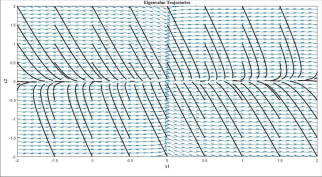 Figure 1
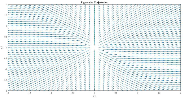 Figure 2
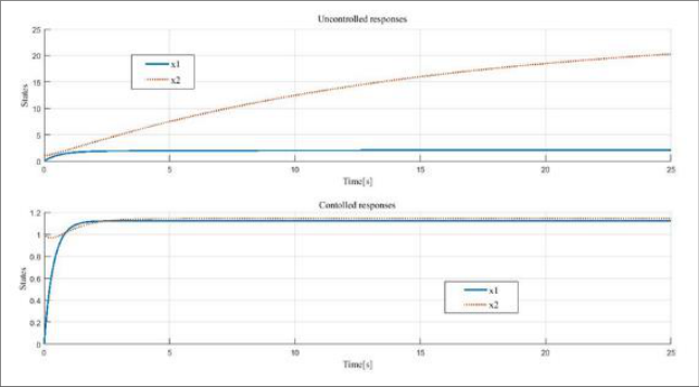 Figure 3
Introduction
It is known in [1,2] that differential equation since its inception from the work on dynamics by Isaac Newton in the mid-17 th century have been known as a major branch of mathematics (pure and applied) which can be used as an instrument for harmonizing different constituents into a single system which might otherwise remain independent of each other in other to analyze the relationships that co-exists between them. Differential equations are vital field of every ongoing investigation with an interesting capability of reformulating basic real world problems and proffering solutions in the various fields. It is one of the most frequent tool used for models in science, economics, engineering and other fields. Mathematical problems for dynamics of changing processes in real world can be modelled into partial or ordinary differential equations depending on the kind of problem under investigation. If some level of unpredictability or randomness is allowed into the system model such as environmental epidemic effects that cannot be effectively estimated, then an all-encompassing mathematical model of the situation or problem according to [3] is a stochastic differential model. It has been assumed that investors decisions are primarily affected by their expected returns, these decisions can be made realistic if a differential equation model that could consider the environmental effects in their decisions is developed as a stochastic parameter in the equation. Stochastic ordinary differential equations are known powerful mathematical tool used for stock price predictions. However, accuracy of stochastic differential equation prediction of stock market prices may be obtained when the drift and the volatility parameters are structured as continuous random variables in the stochastic process instead of constant parameters in the model [4] . Gibbs. J. W, introduced the concept of stochastic processes in 1902 for conversation system with random initial state in statistical mechanics using Hamilton-Jacobi differential equation see [5] . Stochastic processes can be used as a model for systems and phenomena in forecasting any random dynamical behaviors. For example, it is known in [6] that, problems in social, physical and biological sciences where processes of system dynamics are difficult to be described can base their analysis from stochastic point of view rather than a deterministic one. Also, the modelling of price progression for assets with price volatility resulting from some probability and random processes with geometric random motion [7] can base their analysis from stochastic point of view. In recent years, challenges in stock market has led fund managers to work-out convenient ways of raising various investment styles due to the unstable nature and other market factors to enable them predict the fluctuation in stock prices, catch the attention of corporative owners and investors in the stock market to consider liquidity on stock return in their cooperation and not risk and efficiency alone [8] . Stock price fluctuations in the stock market are known to be a reflection of the random movements of their values overtime; these movements and other market anomalies has attracted lots of independent researchers in the industries as well as academia (see for example) [9,10] which helped in the development of Black Scholes equation [11] in the early nineteen-seventies. The development of the Black-Scholes equation by Fischer Black and Myron Scholes in their publication of option pricing model in the early 1970s which later became the foundation of financial market analysis and corner stone of all pricing models whose derivatives can be determined with stocks as an underlying asset [12][13][14][15] is one of the major innovation in stock market history which later became the Black-Scholes model. Several other models including the jump diffusion, Markov switching, Heston processes etc., have been developed because of the short coming in the Black Scholes model (see) [3] to capture volatility as a stochastic process with other special features of stock market data especially the financial market. Predicting the volatility of the variables in the stock exchange market would require some stability analysis if there are poor correlation between the market forces. Stock market stability literally means a state where stock transactions synchronizes with or are in proportion with the market in general and are not significantly disrupted; also stock prices do not experience large fluctuations. The stability of a system simply means that a disturbance in the system input does not result in considerable changes in the system output. Several methods of analysis according to [15] are available including; the fixed point, spectral radius and Lyapunov methods see [2,16,17] , and other references for details). Researchers have shown a renewed interest in analyzing the unstable stock market variables in recent years (see) [3,4,18] to enable owners of cooperation and investors decide on what level of investment to engage on in the stock exchange market. Even though advocates of Efficient Market Hypothesis (EMF) have claimed that technical analysis has little or no correlation with theoretical one, there are lots of literatures according to [19] showing significant correlation between these analysis. The control community is one research group that is addressing the correlation between theoretical and statistical analysis through popular models from feedback control methods. However, financial market analysts are not just interested on stock market stability but desires to find a control measure that would robustly stabilize the market forces and ensure adequate securities with lower cost of purchase. Stability of systems is very much linked to control systems; any device that can manages commands, directs them or can regulate behavior of other systems or devices can be seen as a control system. Controllability, roughly speaking means the possibility of switching a dynamical system from any feasible initial state trajectory to any feasible future state trajectory in the behavior of the system after some finite time using a set of admissible controls; this implies, some systems can be completely controllable. But, if they are not completely controllable then different kinds of controllability concepts such as; null, relative, approximate, constrained controllability [20] etc., can be considered. The novel interest in this research is null controllability; finding a possibility of steering any suitable past state trajectory in the behavior of the system to the origin using an appropriate set of admissible control input as with time. Many researchers [1,[20][21][22][23] have investigated the null controllability of systems and independent results obtained. For example, in [20] , Sathiyaraj et al., presented null controllability criteria for stochastic equations with delay through a rank correlation and perturbed controllability matrix in their investigation of controllability for stochastic equations with delay in finite dimensional spaces. Davies and Oliver [21] investigated the null controllability for neutral type equation having infinite delays where they developed criteria that are sufficient for the control input values to lie in an 𝑛-dimensional unit cube. These criteria guaranteed the null controllable of the system with constraints by the uniform asymptotic stability for the uncontrolled system and full rank condition of the system with control. Motivated by the stochastic analysis works of [3,4] where the unstable nature and some considerable market factors like stock volatility, liquidity of stock return, the drift and spot price in the stock exchange market were analyzed, this paper seeks to improve and extend the works in [3] by investigating the stability and controllability analysis of stochastic model for stock market price. The remaining parts of this research paper is arranged in the following order: The preliminaries, mathematical notations, model formulation and definitions are given in Section 2. The main result on stability is given in Section 3; in the form of theorems and proves while Section 4 presents null asymptotic controllability results for the system. Finally, numerical examples for the theoretical results are presented in Section 5 before Section 6 which contains the discussion and conclusion.
Model Formulation, Preliminaries and Definitions
This section presents some preliminaries and definitions upon which the research hinges and to aid the formulation of the required model.
Preliminaries and Model Formulation
Consider the stochastic volatility model (see) [3] having a just in time (JIT) stock control system with a re-order lead time where the volatility of returns is of the form;
where 𝑆 𝑡 is the stock price process, 𝜇 𝑡 is the drift coefficient of stock price process, 𝑈 𝑡 is the introduced stock control process with coefficient 𝜅 𝑡 , 𝜎 𝑡 is a volatility process considered to be positive and 𝑤 𝑡 is the Weiner process.
A vector valued controlled stochastic differential equation model is developed following the assumptions in [3] and is given by;
with 𝑥 = (𝑆 1 , ⋯ , 𝑆 𝑛 ) 𝑇 , and 𝑢 = (𝑈 1 , ⋯ , 𝑈 𝑛 ) 𝑇 , where 𝑇 denotes the matrix transpose and 𝜎 𝑗𝑖 = 𝜎 (𝑗-(𝑗-1))(𝑖+1) ≠ 0; 𝑖 = 1, ⋯ , 𝑛, 𝑗 = 2, ⋯ , 𝑛.
Let 𝑅 be the real line where 𝐴(𝑡) ∈ 𝑅 𝑛×𝑛 , 𝐵 𝑖 (•) ∈ 𝑅 𝑛×𝑛 are 𝑛 × 𝑛 matrices with 𝐵 𝑖 (𝑡,•) = 0, 𝐶(𝑡) ∈ 𝑅 𝑛×𝑚 , 𝑢 ∈ 𝑅 𝑚 , 𝑥 ∈ 𝑅 𝑛 is the price volatility process, 𝑤 𝑖 (𝑡) ∈ 𝑅 𝑛 is the Weiner processes and 𝑑𝑤 𝑖 (𝑡) its differential form with 𝑑𝑤 𝑖 (𝑡) = 𝜉 𝑡 𝑑𝑡, where 𝜉 𝑡 is a white noise or the correlation coefficient. The vector valued stochastic differential equation model without the control is given by
the future stock price can now be computed from initial data from time 𝑡 using (3) by introducing the transition matrix 𝑋(𝑡) ∈ 𝑅 n×𝑛 (see) [21] . The transition matrix is a continuously differentiable function which is related to the expected rate for correlation of stock prices and returns for trading periods and could reduce risks associated with market volatility; it is defined as
The stock price 𝑥(𝑡) of equation ( 3) can be expressed in the form of integral equation at time 𝑡 by using variation of constant formula (see) [21,24] to get
If 𝐵 𝑖 is assumed to change only at discrete time points 𝑡 𝑖 (𝑖 = 1, ⋯ , 𝑁 -1); 0 = 𝑡 0 < 𝑡 1 < ⋯ < 𝑡 𝑁-1 < 𝑡 𝑁 < ∞, 𝑡 ∈ 𝐽 = [0, ∞), then, the Ito's integral can be used to obtain similar solution as that of (4) see [4]. This research will however not consider the Ito's integral for stochastic processes in the evaluations and analysis. The idea in this paper is to exploit the properties of the transition matrix introduced and assume the Weiner process 𝑤 𝑖 have a correlation only with 𝜉 𝑡 as the correlation coefficient.
Definitions
Some definitions upon which the research hinges will now be given, Definition 1: The opening stock strike price 𝑥 0 (𝑡) of equation ( 3) is said to stable if for every > 0 there exists 𝛿(𝜀) > 0 such that every future stock strike price 𝑥(𝑡) of equation ( 3) with ‖𝑥(0) -𝑥 0 (0)‖ < 𝛿(𝜀) exist and satisfies ‖𝑥(𝑡) -𝑥 0 (𝑡)‖ < 𝜀 on 𝑅.
The initial stock strike price 𝑥 0 (𝑡) of equation ( 3) is said to be asymptotically stable, if it is stable and there exist constant 𝜂 > 0 such that 𝑥(𝑡) -𝑥 0 (𝑡) → 0 as 𝑡 → ∞ whenever ‖𝑥(𝑡) -𝑥 0 (𝑡)‖ ≤ 𝜂 see [3] . Definition 2: The system (3) is asymptotically null controllable if for every initial stock strike price 𝑥 0 ∈ 𝑅 𝑛 there exist a control 𝑢 define on 𝐽 such that 𝑥(0) = 𝑥 0 and lim 𝑥(𝑡) = 0 𝑡 → ∞
Main Results on Stability
Here, some theorems with their proofs are given following [3] as main result on stability in this section.
Theorem 1: Let 𝑋(𝑡) be the transition matrix for equation (3) and 𝑀 > 0, 𝐾 > 0 be constants such that
with ∥ 𝑋(𝑡) ∥≤ 𝑀𝑒 -𝐾 -1 𝑡 , 𝑡 ≥ 0. Furthermore, if
is satisfied with 𝜌 satisfying 0 ≤ 𝜌 < 𝐾 -1 . Then, the opening stock strike price of system (3) is asymptotically stable.
Proof:
The proof is given in [3] and will only be sketched. Let 𝑋(𝑡) be the fundamental matrix of (3) with 𝑋(0) = 𝑥 0 . Then, there exists 𝑀 > 0 a constant such that ∥ 𝑋(𝑡) ∥≤ 𝑀𝑒 -𝑡𝑘 -1 , where 𝑘 > 0 and 𝑡 ≥ 0. Thus 𝑥(𝑡) → 0 as 𝑡 → ∞. If 𝑥(𝑡) is a local solution of equation ( 3) defined to the right of 𝑡 = 0, then, by the variation of parameter formula (4) of the system we get max 0≤𝑠≤𝑡 ‖𝑥(𝑠)‖ ≤ (1 -𝜌𝐾) -1 𝐿 ∥ 𝑥 0 ∥. It follows that ‖𝑥(𝑠)‖ ≤ (1 -𝜌𝐾) -1 𝐿 ∥ 𝑥 0 ∥ as long as 𝑥(𝑡) is defined. That is 𝑥(𝑡) is extendable to +∞ (see) [25] and the initial stock strike price is stable. To show that 𝑥(𝑡) → 0 as 𝑡 → ∞. Let 𝑐 = limsup 𝑡→∞ ‖𝑥(𝑡)‖ and pick 𝑑 such that 𝜌𝐾 < 𝑑 < 1. If 𝑐 > 0, then, since 𝑑 -1 𝑐 > 𝑐, there exists 𝑡 0 ≥ 0 such that ‖𝑥(𝑡)‖ ≥ 𝑑 -1 𝑐 for every 𝑡 ≥ 𝑡 0 . Thus, equation (4) implies ‖𝑋(𝑡)‖‖𝑥 0 ‖ + ‖𝑋(𝑡)‖ ∫ ‖𝑋 -1 (𝑠) ∑ 𝐵 𝑖 (𝑠, 𝑥(𝑠))𝜉 𝑡 𝑛 𝑖=1 ‖ 𝑡 0 0 𝑑𝑠 + 𝜌𝐾𝑑 -1 𝑐. Taking the lim sup as 𝑡 → ∞, we obtain 𝑐 ≤ 𝜌𝐾𝑑 -1 𝑐, this is a contradiction. Thus, 𝑐 = 0 and this completes the proof.
Proposition 1: Let 𝑋(𝑡) be the fundamental matrix of (3) with 𝐵 𝑖 (•) = 0. Then system (3) is stable if and only if there exists 𝐾 > 0 a constant with ‖𝑋(𝑡)‖ ≤ 𝐾, 𝑡 ∈ 𝑅
The system (3) is uniformly stable if and only if there exists 𝐾 > 0 a constant with ‖𝑋(𝑡)‖ ≤ 𝐾, 0 ≤ 𝑠 ≤ 𝑡 < +∞.
The system (3) is uniformly asymptotically stable if and only if there exists 𝐾 > 0, 𝛼 > 0 constants with ‖𝑋(𝑡)𝑋 -1 (𝑡)‖ ≤ 𝐾𝑒 -𝛼(𝑡-𝑠) , 0 ≤ 𝑠 ≤ 𝑡 < +∞.
Proof:
The proof follows similarly like that of [25; P.61] Theorem 2: Let 𝑋(𝑡) be the fundamental matrix of equation ( 3) with 𝐵 𝑖 (•) = 0, such that ‖𝑋(𝑡)𝑋 -1 (𝑡)‖ ≤ 𝐾𝑒 -𝛼(𝑡-𝑠) , 𝑡 ≥ 𝑠 ≥ 0, where 𝐾, 𝛼 are positive constants and let
where 𝜌 is sufficiently small positive constant satisfying 𝜆 < 𝐾 -1 𝜌, now if 𝑐 = 𝜌 -𝜆𝐾, then every solution 𝑥(𝑡) of ( 3) defined to in a right neighborhood of 𝑡 0 with 𝑡 ≥ 𝑡 0 satisfying ‖𝑥(𝑡)‖ ≤ 𝐾𝑒 -𝑐(𝑡-𝑠) ‖𝑥(𝑠)‖, for every 𝑡 ≥ 𝑠 ≥ 𝑡 0 is said to be uniformly asymptotically stable Proof: By ( 4 Thus if 𝑧(𝑡) = 𝐾𝑒 -𝜌(𝑡-𝑡 0 ) ‖𝑥(𝑡)‖ we have
By applying the Grownwall's inequality we get 𝑧(𝑡) = 𝐾𝑧(𝑡 0 )𝑒 -𝜆𝐾(𝑡-𝑡 0 ) for 𝑡 ≥ 𝑡 0 , and ‖𝑥(𝑡)‖ = 𝐾‖𝑥(𝑡 0 )‖𝑒 -𝑐(𝑡-𝑡 0 ) . This implies 𝑥(𝑡) is continuable to +∞.
Controllability Results
In this section, we study controllability of the system when some control measures are introduced into the vector valued stochastic volatility model. The control equation of ( 3) is given by ( 2 Here the matrices 𝐴, C and 𝐵 𝑖 are as defined in Subsection 2.1. The solution of (2) can be obtained following the methods in [26] by Defining 𝑋(𝑡) = 𝑋(𝑡, 𝑡 0 ), then 𝑋(𝑡, 𝑡 0 ) = 𝑋(𝑡)𝑋 -1 (𝑡 0 ) to get
Define 𝑌(𝑠) = 𝑋(𝑡, 𝑠)𝐶(𝑠) and the controllability matrix
where T denotes the transpose of the matrix. We assume that the following limits exists;
Main Result on Asymptotic Null Controllability
Here, the main result on asymptotic null controllability of the system is stated with proof.
Theorem 3: System (2) is asymptotically null controllable if and only if 𝑊 is nonsingular. Proof: Assume first that 𝑊 is nonsingular, so that each 𝑢(𝑡) defined on [0, 𝑡 1 ] is given by;
𝐵 𝑖 (𝑠)𝜉 𝑡 (𝑠)𝑑𝑠). Clearly 𝑥(0) = 𝑥 0 with lim 𝑡→∞ 𝑥(𝑡) = 0 and system (2) is asymptotically null controllable; where 𝑥 is the solution of equation ( 2) which corresponds to the input control 𝑢.
Assume for a converse that 𝑊; the controllability matrix is singular. Then, there is a vector 𝑣 ≠ 0, such that 𝑣𝑊𝑣 𝑇 = 0. So that ∫ 𝑣𝑌(𝑠)(𝑣𝑌(𝑠)) 𝑇 ∞ 0 𝑑𝑠 = 0. Therefore, 𝑣𝑌(𝑠) = 0 almost everywhere for 𝑠 ∈ 𝑅. The asymptotically null controllable of the solution implies the existence a control 𝑢(•) such that
Letting 𝜉 𝑡 = 0, we have 𝑋(𝑡)𝑥 0 + ∫ 𝑌(𝑠) ∞ 0 𝑢(𝑠)𝑑𝑠 = 0. It follows that 𝑣𝑋(𝑡)𝑥 0 + ∫ 𝑣𝑌(𝑠) ∞ 0 𝑢(𝑠)𝑑𝑠 = 0, which implies that 𝑣𝑋𝑥 0 = 0. Since 𝑋 ≠ 0 and 𝑥 0 ≠ 0, it follows that 𝑣 = 0, which contradicts the fact that 𝑣 ≠ 0. Therefore, W is nonsingular.
Example
In this section, a two dimensional stochastic differential equation model is given as example. Consider the volatility model;
This can be written in matrix form 𝑑𝑥(𝑡) = 𝐴(𝑡)𝑥(𝑡)𝑑𝑡 + 𝐶(𝑡)𝑢(𝑡) + ∑ 𝐵 𝑖 (𝑡, 𝑥(𝑡))𝑑𝑤 𝑖 (𝑡) 2 𝑖=1
where the processes 𝑆 1 (𝑡), 𝑆 2 (𝑡) are correlated with 𝜎 21 = 𝜎 12 ≠ 0 and 𝐵 1 (𝑡) = ( 𝜎 11 0 0 𝜎 21 ) , 𝐵 2 (𝑡) = ( 𝜎 12 0 0 𝜎 22 ).
Data Analysis and Result
In this section, eighteen years stock exchange market (1997-2014) from the Nigerian exchange market (NSE) were extracted from [4] with initial stock prices, volatility, trading days and drift to illustrate its nature. The values to be used in this subsection were calculated in details using stock returns over a period with the appropriate allocation as given in [3] .
Illustration of asymptotic Stability Result
The volatility matrix 𝐵 𝑖 , 𝑖 = 1, 2 in equation (10) with 𝑢 = 0, is given by with eigenvalues 𝜆 = -0.0681, -1.6288 and the transition matrix of system (10) is obtained by the method in [21] as 𝑋(𝑡) = ( 0.0182𝑒 -0.0681𝑡 0.0182𝑒 -1.6288 𝑡 1.5559𝑒 -0.0681𝑡 -0.0048𝑒 -1.6288 𝑡 )
The stability of system (10) with 𝑢 = 0 can be found using Condition (i) and Condition (ii) of Theorem 1 as follows: By Condition (i);
∫ ‖( 0.0182𝑒 -14.6843𝑡 0.0182𝑒 -0.6140 𝑡 1.5559𝑒 -14.6843𝑡 -0.0048𝑒 -0.6140 𝑡 ) ( 0.0115𝑒 -14.6843𝑠 0.0437𝑒 -14.6843 𝑠 89.2267𝑒 -0.6140𝑠 -1.0438𝑒 -0.6140 𝑠 )‖ 𝑑𝑠 Observe, that some conditions of Theorem 1 are not satisfied; for example 0 ≤ 𝜌 ≮ 𝑘 -1 . This implies, the stock price data of the NSE extracted and used in for this model is not asymptotically stable. Hence, the system (10) with 𝑢 = 0 is not asymptotically stable.
Illustration on Asymptotic Null Controllability Result
Consider system (10) where To prove asymptotic null controllability result for system (10) using the NSE data from [4], is to show the non-singularity of the controllability matrix by Theorem 3 as follows. Let 𝑌(𝑠) = 𝑋(𝑡, 𝑠)𝐶(𝑠), with 𝑋(𝑡, 𝑠) as given by (11). So that 𝑌(𝑠) = 𝑋(𝑡, 𝑠)𝐶(𝑠) = ( 0.0728𝑒 -0.0681𝑡 0.0728𝑒 -1.6288𝑡 6.2236𝑒 -0.0681𝑡 -0.0192𝑒 - So that the determinant of the controllability matrix |𝑊| = 0.2065 and is nonsingular. This implies the system (10) is asymptotically null controllable.
Discussion and Conclusion 6.1 Discussion
In [3] , the effects of stochastic volatility on the stability of stock market and expected return on normal distribution were discussed. It was known that, stochastic volatility has a leverage effect on the size of the tails and skewness of the return distribution. However, when the volatility 𝜎 and 𝜉 𝑡 , the correlation coefficient which indicates the origin of randomness for the underpinning Weiner process are absent. That is, if 𝜎 = 0; the volatility becomes deterministic giving a stable market phase because ∑ 𝐵 𝑖 (•) will be zero, this leads to a normally distributed stock returns like that of Black Scholes model. In this paper, we have used the vector valued controlled stochastic differential model given by ( 2) to analyze stability and controllability of the dynamics such as expected return, liquidity on stock return and other market conditions in the financial market. The stability dynamics of the stochastic model given by (3) was analyzed using Theorem 1 and 2 where the stock price solution to the stochastic model was used to develop and analyze conditions under which the random price of stock in the financial market would become stable.
The analysis of the stock market using data obtained from Adeosun et al., [4] shows price stability within the trading periods which is expected from the NSE when volatility becomes deterministic because the processes 𝐵 𝑖 and 𝑢 are assumed to be zero in system (10), giving a stable market phase as seen in the phase portraits Figure 1. The trajectories of eigenvectors which are a function of the drift from infinite-distance, moves towards the critical point and converges at that point. That is, they move directly towards the critical point and converge at it when the eigenvalues of the trajectories are less than zero. However, using the same data on system (10) with 𝑢 = 0 shows price instability; this is an anticipated outcome of a stock market trade with volatility of the stock under various random features as shown in Figure 2. In Figure 3, an open loop response showing asymptotic null controllability of system (10) is presented using same data but with some effective stock control measures. This implies random prices of stock in the stock market would become stable if for every initial expected rate of share price change in the stock market. There is a control measure defined on the randomness of the stochastic trading period such that, the solution (which is the stock market prices) at the initial trading in the floor of the stock market is the initial expected rate of share price, and the price remains the same at the close of the trading periods.
Conclusion
In this research paper, results for stability and controllability for stock exchange market were obtained; first by developing a vector valued stochastic differential system with control. The stability analysis was obtained by utilizing the characteristics of the transition matrix solution for the vector valued system with some boundedness condition placed on the stochastic part. The controllability result is then obtained with respect to the nonsingularity of the controllability matrix which is a function of the drift. Illustrative examples on the effectiveness of the theoretical analysis of the model are given and simulation output results presented using MATLAB.
References
26 in the original paper- Davies I. Euclidean Null Controllability of Infinite Neutral Differential Systems, Anziam J. 2006;48(2):285-293.
- Davies I, Haas OLC. Robust Guaranteed Cost Control for a Nonlinear Neutral System with Infinite Delay," in European Control Conference. 2015;1:1255-1260.
- Davies I, Uchenna AI, NDURI. Stability Analysis of Stochastic Model for Stock Market Prices, Int. J Math. Comput. Methods. 2019;4:79-86.
- Adeosun ME, Edeke SO, Ugbebor OO. Stochastic analysis of stock market price models: A case study of the Nigeria stock exchange (NSE)," WSEAS Trans. Math. 2015;14:353-363.
- Mao X. A Note on the LaSalle-Type Theorems for Stochastic Differential Delay Equations, J Math. Anal. Appl. 2002;268:125-142, doi: 10.1006/jmaa.2001.7803.
- Mao X. Robustness of Stochastic Differential Delay Equations with Markovian Switching, SACTA. 2000;3(1):48-61.
- Osu BO. A Stochastic Model of the Variation of the Capital market Price," Int. J. Trade, Econ. Financ. 2010;1(3):297-302.
- Shammakhi HR, Mehrabi A. Study the Effect of Liquidity of Stock on Stock Returns in the Companies Listed in Tehran Stock Exchange, Int. J Econ. Commer. Manag. 2016;IV(12):423-434.
- Osborn MFM. Browmian motion in the stock market operations research, Ind. Manag. Rev. 1965;6:13-32.
- Samuelson P. Economics theorem and mathematics -An appraisal cowls foundation paper 61, Repr. Am. Econ. Rev., vol. 1952;42:56-69.
- Black F, Scholes M. Valuation of options and corporate liabilities, J. Polit. Econ., 1973;81:637-654.
- Liu XL. Stochastic Process and its Role in The Development of the Financial Market: Celebrating Professor Chows Long and Successful Career, Commun. Stoch. Anal. 2019;13(3):1-9. doi: 10.31390/cosa.13.3.07.
- Mondal MK, Alim A, Rahman F, Biswas HA. Mathematical Analysis of Financial Model on Market Price with Stochastic Volatility, J Math. Financ. 2017;7:351-365doi: 10.4236/jmf.2017.72019.
- Biswas HA. On the Evolution of AIDS / HIV Treatment : An Optimal Control Approach, Curr. HIV Res. 2014;12:1-12.
- Davies I, Ebiwareme L, Ekesiobi OI, Brown-ikiri PE, Nnaa F. Stability and Feedback Control of Volterra Type Systems with Time Delay, Asian Research Journal of Mathematics. 2022;18(12):1-15. Doi:10.9734/ARJOM/2022/v18i12620.
- Lucky AC, Davies I, Stanley CT, Humphrey AE. Stability and Feedback Control of Nonlinear Systems, International Journal of Control Science and Engineering. 2020;10(1):11-15.
- Davies I, Haas OCL. Delay-Independent Closed-Loop Stabilization of Neutral Systems with Infinite Delays," Technol. Int. J. Math. Comput. Phys. Electr. Comput. Eng. 2015;9(9):496-50.
- Gardini L, Radi D, Schmitt N, Sushko I, Westerhoff F. Causes of Fragile Stock Market Stability, J Econ. Behav. Organ. 2022;200:483-498.
- Samad T, Annaswamy AM. The Impact of Control Technology, 2 nd ed. United States: IEEE Control Systems Society and the American Automatic Control Council, 2014.
- Sathiyaraj T, Michal F, Wang J. Null controllability results for stochastic delay systems with delayed perturbation of matrices, Chaos, Solitons and Fractals. 2020;138:1-12. doi: 10.1016/j.chaos.2020.109927.
- Davies I, Haas OC. Null controllability of neutral system with infinite delays, Eur. J Control. 2015;26:28-34. doi: 10.1016/j.ejcon.2015.09.001.
- Davies I. Euclidean null controllability of linear systems with delays in state and control, J Niger. Assoc. Math. Phys. 2006;10:553-558,.
- Chukwumela A, Davies I, Nwaoburu AO. Euclidean Controllability of Linear Systems with Delayed State and Control Variables. Asian Journal of Pure and Applied Mathematics. 2023;5:289-297.
- Cotterell TS, Davies I, Abraham CL. Stability and Controllability of Nonlinear Systems, Asian J. Math. 2020;16(2):51-60.
- Kartsatos AG. Advanced Ordinary Differential Equations. Tampa, Florida: Mariner Publishing Company, Inc, 1980.
- Davies I, Jackreece P. Controllability and null controllability of linear systems, J Appl. Sci. Environ. Manag. 2005;9(3):3136.
Cited by 2
From OpenAlex, OpenCitations and reference lists read by Scinovex
- Effect of Time Delay in the Stability Analysis of Cholera Epidemic-Endemic Disease Model ↗
Adiela Chukwumela, Iyai Davies · European Journal of Theoretical and Applied Sciences · 2024
Cholera as a disease is a kind of acute diarrhea caused by bacteria Vibrio cholerae. A nonlinear delayed mathematical model with environmental factor for the spread of infectious disease cholera is proposed and analyzed. A mathematical model for cholera was improved by adding a time delay that represents the time between the instant at which an individual becomes infected and…
❝ 2PDF - Application of Non-Linear Evolution Stochastic Equations with Asymptotic Null Controllability Analysis ↗
I.U. Amadi, Love Cherukei Nnoka, Chimaobi Amadi · International Journal of Mathematics and Statistics Studies · 2024
This paper investigated system of stochastic differential equations with prominence on disparities of drift parameters. These problems were solved analytical by adopting the Ito’s method of solution and three different investment solutions were obtained consequently. The necessary conditions were achieved which govern various drift parameters in assessing financial markets. Therefore, the impressions on each solution of investors in financial markets…
❝ 0PDF