
Research article · 2023 · Full text
International Journal of Statistics and Applied MathematicsEvaluation of statistical models for rainfall at rars: Jagitial
Volume 8(4) · Pages 26–35 · DOI: 10.22271/maths.2023.v8.i4a.1076 ↗
Research areasAgricultural Economics and PracticesHydrology and Drought Analysis
Abstract
Author-writtenIn general, the amount of rainfall and its frequency impacts agricultural, ecological, hydrological, economic and living systems. Rainfall is one of the important factors in agriculture. It plays a major role in the growth and development of the crop starting from germination to harvesting. Change in pattern of rainfall will lead to unexpected responses from plant. Thus, farmers in India were facing problems, as most of the crops grown under rainfed condition. Since precipitation is unpredictable, the present study was undertaken to analyse the distribution pattern of rainfall and to know effect of other weather parameters like maximum and minimum temperature, relative humidity, evaporation etc. on rainfall. The latest 31 years secondary data pertaining to weather parameters was collected from RARS, Jagitial, Telangana. For the convenience of analysis data has been divided into 3 major data sets viz. Annual, Monsoon seasonal months and Standard Meteorological weeks. The results based on Kolmogorov Smirnov and RMSE tests indicated Exponential distribution was best fitted distribution for most of the data sets. Exponential distribution was best fit for annual and seasonal months, while for SMW’s Exponential and Pearson type III were best fitted.
Summary
Source-checkedPlain-language reading of the full paper, prepared with AI and checked against the text. Each point links to the authors' own words.
Why it matters
- Rainfall is a critical factor in agriculture, influencing crop growth and development from germination through to harvest. View evidence ↗
- Variability in rainfall can impact regional economies, water supplies, transportation, and overall agricultural production. View evidence ↗
- While extreme rainfall damage cannot be fully avoided, analyzing rainfall data can provide useful forewarnings. View evidence ↗
The question
- The study aimed to analyze rainfall distribution patterns and determine the effects of other weather parameters, such as temperature and humidity, on rainfall. View evidence ↗
What they did
- The research used 30 years of secondary weather data (1988-2018) collected from the Regional Agricultural Research Station in Polasa, Jagitial. View evidence ↗
- Rainfall data was divided into 24 sets, including annual, seasonal (Monsoon and Post Monsoon), monthly (June-September), and 17 Standard Meteorological Weeks (SMW 23-39). View evidence ↗
- The study evaluated several probability distributions to find the best fit, including Log Normal, GEV, Weibull, Gumbel, and Pearson type III. View evidence ↗
- The Kolmogorov-Smirnov (KS) test and Root Mean Square Error (RMSE) were used to identify the best-fitted distributions. View evidence ↗
What they found
- The mean rainfall was 859.21 mm annually, 708.36 mm for seasonal months, and 87.62 mm for the Post Monsoon period. View evidence ↗
- The coefficient of variation (CV) was 34.55% for annual data and 34.72% for the monsoon season, while SMW variation ranged from 85.16% to 162.45%. View evidence ↗
- For annual, monsoon, and post-monsoon datasets, the Exponential distribution was the best fit according to the KS test, with p-values of 0.93, 0.95, and 0.84 respectively. View evidence ↗
- The Exponential distribution best described rainfall for June, July, and September, while the Log Normal distribution was the best fit for August (p-value 0.54). View evidence ↗
- The Exponential distribution was the best fit for most Standard Meteorological Weeks, though Pearson type III was best for the 23rd, 37th, and 38th SMWs. View evidence ↗
- RMSE values for SMWs ranged from 33 to 92, with the lowest value of 33.77 observed for the 39th SMW using the Exponential distribution. View evidence ↗
What it means
- The authors concluded that the Exponential distribution was widely the best fit for almost all analyzed rainfall datasets. View evidence ↗
Figures & tables
From the original paper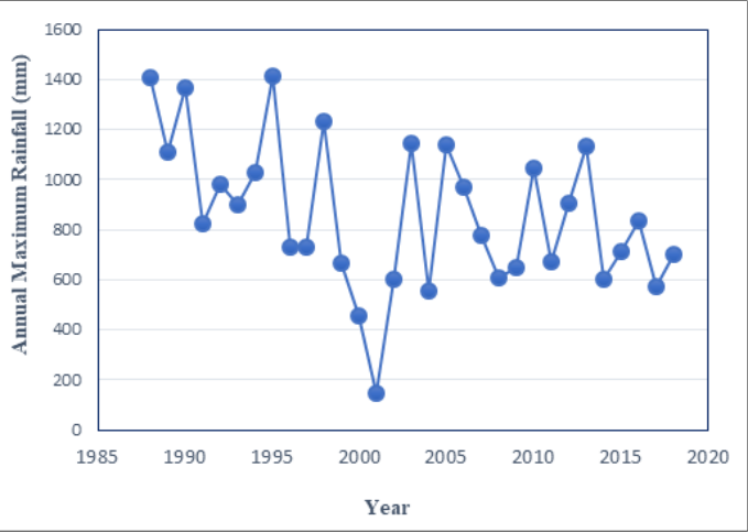 Figure 1
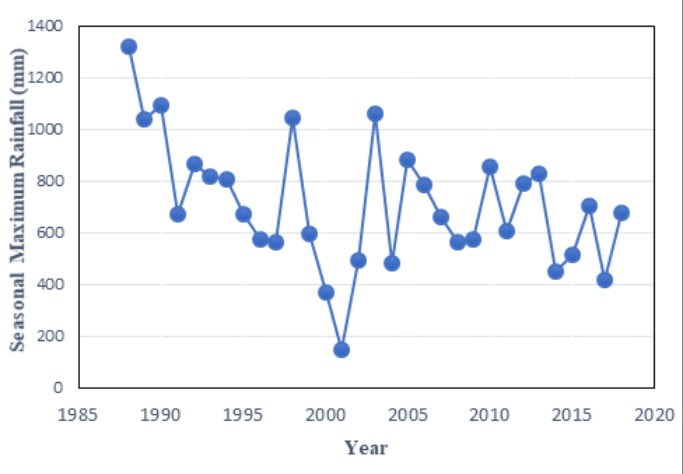 Figure 2
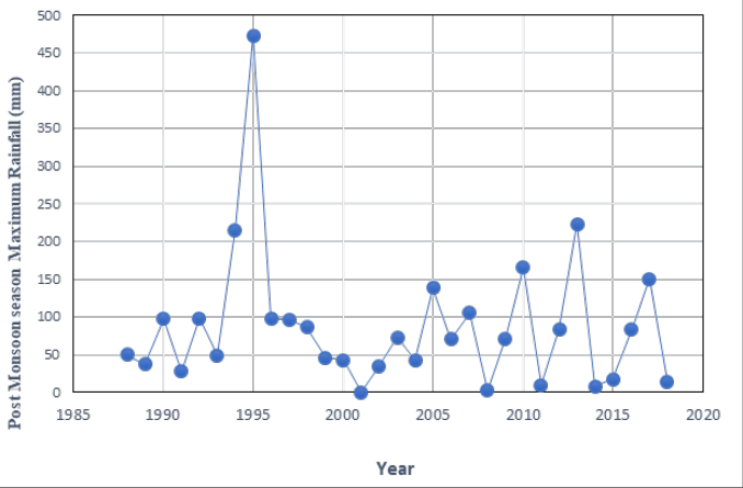 Figure 3
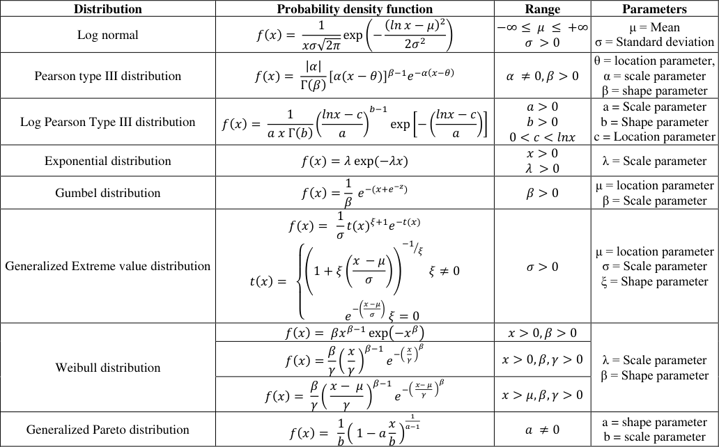 Table 1
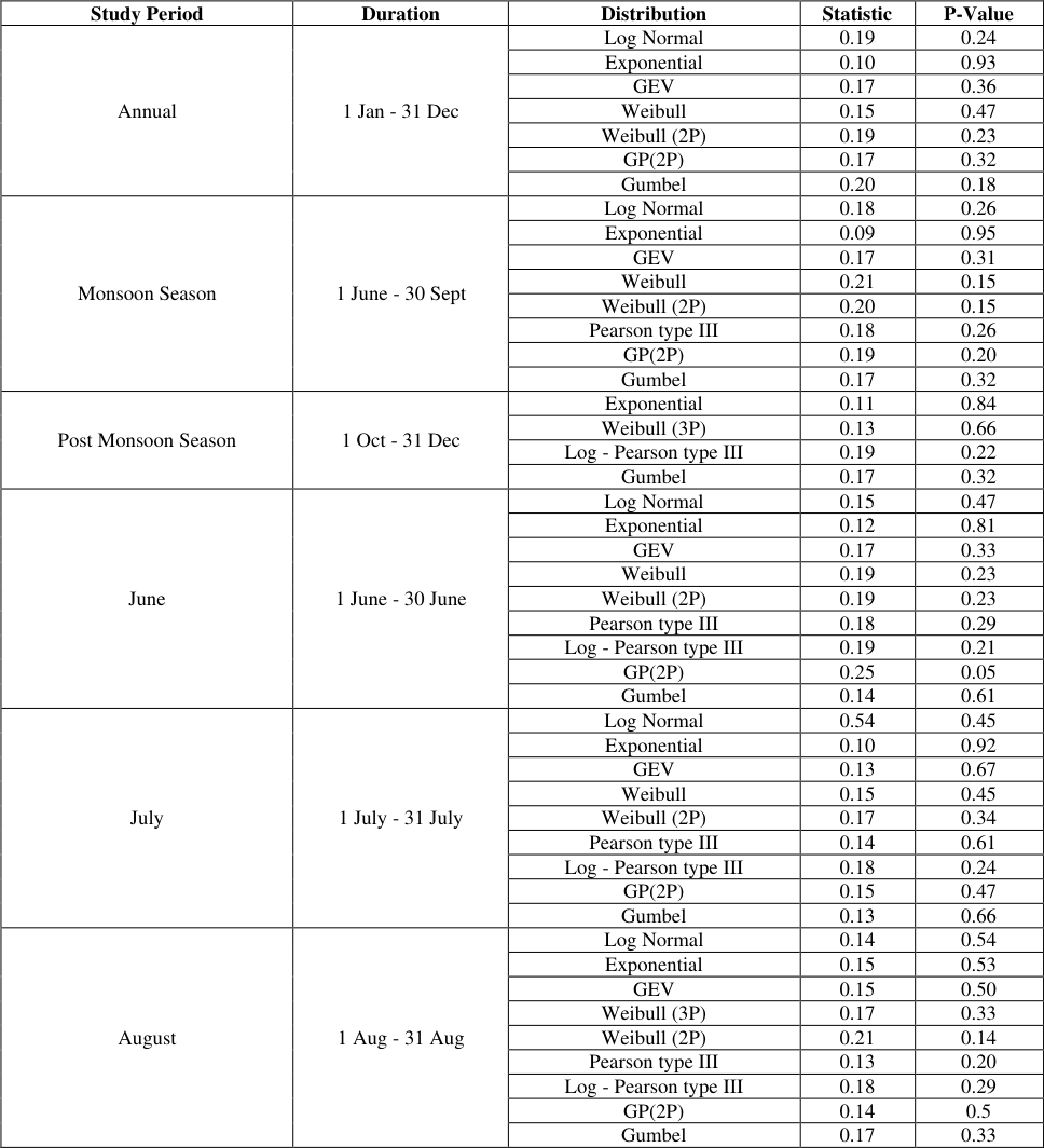 Table 2
 Table 3
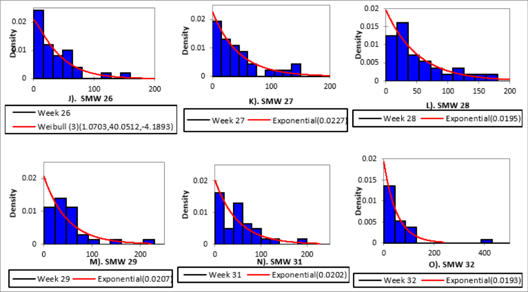 Figure 4
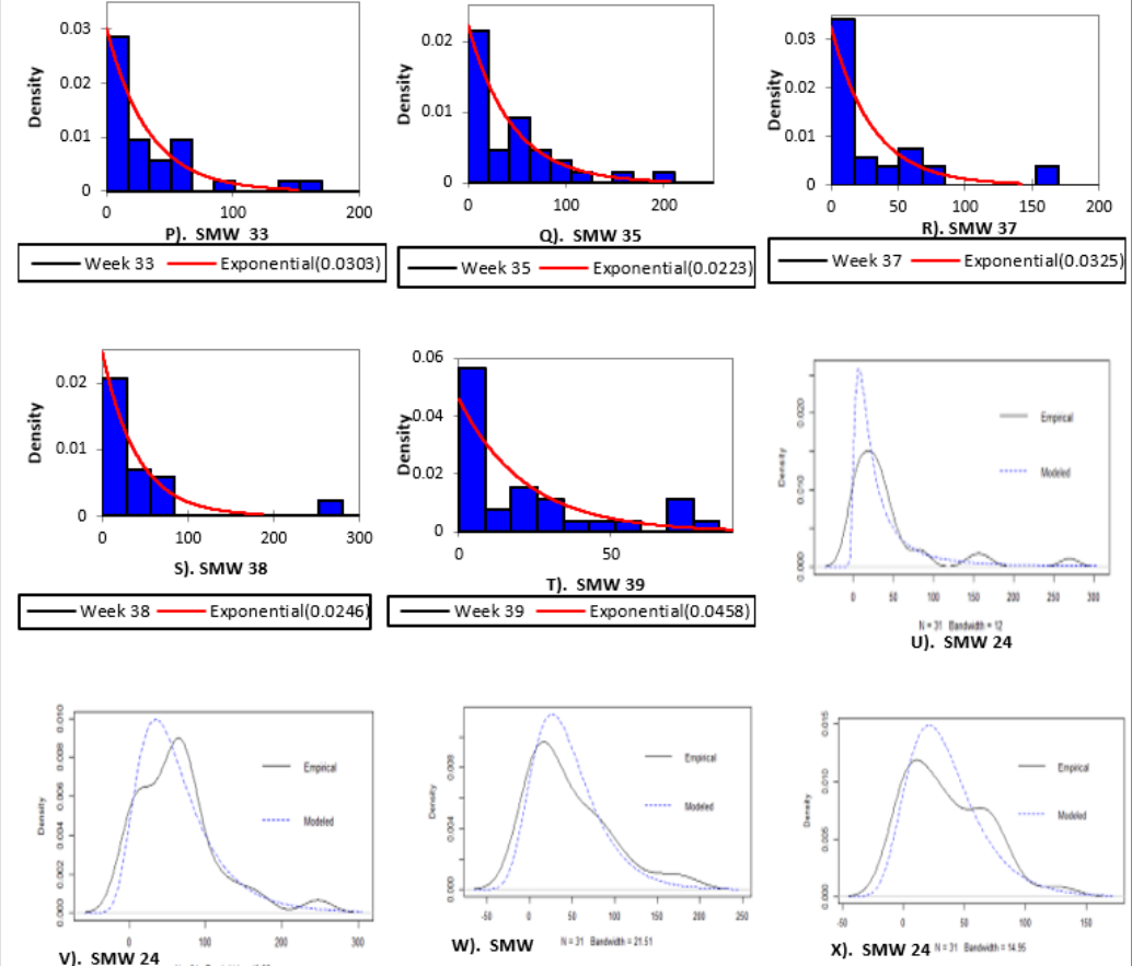 Figure 5
Introduction
Rainfall intensity, duration and its distribution play a major role in the growth of agriculture and other related sectors and the overall development of a country. The variability in rainfall affects the agricultural production, water supply, transportation, the entire economy of a region, and the existence of its people. In regions where the year-to-year variability is high, people often suffer great calamities due to floods or droughts. The damage due to extremes of rainfall cannot be avoided completely, a forewarning could certainly be useful and it's possible from analysis of rainfall data. The prediction of rainfall at a particular place and time can be made by studying the behaviour of rainfall of that place over several years during the past. This behaviour is best studied by fitting a suitable distribution to the time series data on the rainfall (Kainth 1996) [5] . Alam MA, et al. (2018) [1] , aimed to determine the best-fit probability distributions in the case of maximum monthly rainfall using 30 years of data (1984-2013) from 35 locations in Bangladesh by using different statistical analysis and distribution types. Generalized Extreme Value, Pearson type 3 and Log-Pearson type 3 distributions showed the largest number of bestfit results. Among the best score results, Generalized Extreme Value yielded the best-fit for 36% of the stations and Pearson type 3 and Log-Pearson type 3 each yielded the best-fit for 26% of the stations. Młyński D, et al. (2019) [8] , studied to determine the best probability distributions for calculating the maximum annual daily precipitation with the specific probability of exceedance. The Root Mean Square Error (RMSE), and the coefficient of determination (R 2 ) were used for assessing the fit of empirical and theoretical distributions. They identified that the GEV distribution -recommended for calculating the maximum daily precipitation with the specific probability of exceedance in the catchments of the upper Vistula Basin.
The study on statistical analysis of rainfall may help the government in agricultural planning and policy making, it helps farmers in contingency planning of the crop, adopting the farm production practices, management of the farm production etc. (Husak et al., 2007) [4] . The present study focusses on fitting appropriate Statistical distributions for rainfall data. Thus to understand the distribution of rainfall in RARS, Jagitial region for better agricultural management.
Data and Study area
Telangana is classified as a semi-arid state and mean yearly rainfall varies from 677 mm to 998 mm (Waghaye, et al., 2018) [9] . The present study was conducted to know the rainfall variability in and around the region of the Regional Agricultural Research Station, (RARS). The station is located at Polasa village of Jagitial district of Telangana State. It belongs to the Northern Telangana zone of Telangana. The geographical co-ordinates of the station are Latitude: 18-49' 40" North Longitude: 78-56' 45" East. The present study was based on the secondary data on weather parameters over a period of 30 years (1988-2018) which was collected from Regional Agricultural Research Station, Polasa, Jagitial.
Methodology 3.1 Fitting Probability distributions
Rainfall is highly variable in a given period. Hence, there is a need to study the distribution both on long term (annually or seasonally) as well as short term (monthly or weekly) basis. Among the weather parameters, amount of daily maximum rainfall (mm) was considered to fit appropriate probability distributions. The probability distributions viz., log normal, Gamma, Generalized extreme value (GEV), Weibull (1 P, 2 P, 3 P), Gumbel, Generalized Pareto, Pearson type III and Log -Pearson type III were used to evaluate the best fit probability distribution for rainfall.
Description of parameters 3.2.1 Shape parameter
Shape parameters allow a distribution to take on a variety of shapes, depending on the value of the shape parameter. These distributions are particularly useful in modelling applications since they are flexible enough to model a variety of data sets. Examples of shape parameters are skewness and kurtosis.
Scale parameter
In probability theory and statistics, a scale parameter is a special kind of numerical parameter of a parametric family of probability distributions. The larger the scale parameter, the more spread out the distribution. In general, a scale parameter stretches or squeezes a graph. The examples of scale parameters include variance and standard deviation.
Location parameter
The location parameter determines the position of central tendency of the distribution along the x-axis. A location family is a set of probability distributions where µ is the location parameter. The location parameter defines the shift of the data. A positive location value shifts the distribution to the right, while a negative location value shifts the data distribution to the left. Examples of location parameters include the mean, median, and the mode. A shape-dominated regime describes a pattern where the rainfall tends to be symmetrically distributed, indicating that drier-than-average events are as common as wetter-thanaverage events. Scale-dominated rainfall describes locations where the variance is quite large in comparison to the mean.
Testing for goodness of fit
The goodness of fit test measures the discrepancy between observed values and expected values. Kolmogorov-Smirnov test was used to test for the goodness of fit. In the present investigation, the goodness of fit test was conducted at α = 0.05 level of significance. It was applied for testing the following hypothesis: H0: The maximum daily rainfall data follows a specified distribution. H1: The maximum daily rainfall data does not follow a specified distribution.
Kolmogorov-Smirnov test (K-S test)
This test was used to decide whether a sample comes from a hypothesized continuous PDF. The KS test compares the cumulative distribution functions of the theoretical distributionthe distribution described by the estimated shape and scale parameterswith the observed values and returns the maximum difference between these two cumulative distributions (Wilks, 1995) [10] . This maximum difference in cumulative distribution functions is frequently referred to as the KS statistic. It is based on the empirical distribution function i.e., on the largest vertical difference between the theoretical and empirical cumulative distribution functions which is given as:
Where, 𝑋 𝑖 = Random sample, I = 1, 2 … n.
The frequency density at different levels of rainfall was calculated using the following formulae.
Relative Frequency =
Relative Frequency =
Class frequency
Class frequency
Frequency Density =
Relative frequency Class width
Root Mean Square Error (RMSE)
Root Mean square Error is the standard deviation of the residuals (Prediction errors). It tells about how concentrated the data is around the line best fit. Root Mean error is commonly used in climatology, forecasting and regression analysis to verify experimental results.
𝑁 Where, (𝑍 𝑓𝑖 -𝑍 𝑜𝑖 ) 2 Are squared differences, and N is the sample size.
Results and Discussion
The weather data of Regional Agricultural Research Station, Jagitial had been collected for 31 years (1988-2018) and were analysed by different statistical tools for achieving the previously stated objectives. The results of the study were shown under the following headings: 2 shows the variation in rainfall during the monsoon season, varying between 149 mm to 1319 mm. Similarly, Fig. 3 represents the variation in Post Monsoon season maximum daily rainfall. The highest peak was shown during the year 1995 which was about 417 mm and minimum was during the year 2001 when no rains were received.
Fitting of probability distributions
The distributions used to estimate the best fit for rainfall were Log Normal, Exponential, Generalized Extreme Value (GEV), Weibull (1P, 2P, 3P), Gumbel, Pearson type III (P -III), Log Pearson type III (LP -III), and Generalized Pareto (GP). Goodness of fit for different probability distributions was examined using three tests which are as follows:
1. Root Mean Square Error 2. II. Kolmogorov -Smirnov test (KS test)
The test statistic values along with the pvalues for each data set was computed for the probability distributions mentioned earlier.
The results of analysis are grouped into three groups and presented as follows:
A. Annual and Seasonal datasets
This section consists of three datasets which include Annual, Monsoon and Post monsoon datasets. For all the data sets in this section the best fitted distribution as shown by KS test is Exponential distribution. The KS test statistic values of the three data sets were 0.10, 0.09 and 0.11 with P-Values of 0.93, 0.95, 0.84 respectively. Among all the three data sets Exponential distribution best describes the Monsoon data set which has the least KS test statistic with highest pvalue. The graphs of the best fitted distributions were shown in the Fig. 4. From the graphs we can infer that one parameter Exponential distribution described the data well, which was also indicated by the graph shown in Fig. 4 (C).
B. Monsoon Seasonal months
The months considered under this section were June to September. KS test results showed that a total of nine distributions. Fitted for each month under this section. The distribution that did not fit any of the data set under this section was Weibull (1P) distribution. KS test showed that Exponential distribution described well for June, June and September seasonal months, while for August the best fitted distribution was Log Normal distribution with test statistic 0.14 and P-Value 0.54. The test statistic values of Exponential distribution for the month of June, July and September were 0.12, 0.10 and 0.11 with pvalues of 0.81, 0.92 and 0.86 respectively. The parameter estimates of the best fitted distributions were given in the Table 3. The lambda (λ) were 0.0076, 0.0043 and 0.0069 for June, July and September respectively. The parameter estimate of the month of August was 0.0051. Along with parameter estimates the RMSE values of the best fitted distributions were also shown under the same Table . 3. For the 4 monsoon seasonal months the least RMSE value was observed for the month of June month which was of 157.80. The RMSE values for other three months were 265.54, 228.37 and 168.82 respectively. The best fitted distribution graphs for the monsoon months were shown in Fig. 4 (D-G).
| Study Period | Range | Distribution | Location | Scale | Shape | RMSE value |
|---|---|---|---|---|---|---|
| Annual | 1 Jan - 31 Dec | Exponential | λ = 0.0012 | 907.49 | ||
| Monsoon | 1 June - 30 Sept | Exponential | λ = 0.0014 | 710.06 | ||
| Post Monsoon | 1 Oct - 31 Dec | Exponential | λ = 0.0114 | 125.71 | ||
| June | 1 June - 30 June | Exponential | λ = 0.0 076 | 157.80 | ||
| July | 1 July - 31 July | Exponential | λ = 0.0043 | 265.54 | ||
| August | 1 Aug - 31 Aug | Log Normal | λ = 0.0051 | 228.37 |
Table text extracted from the original PDF; superscript letters are shown inline. The original table image is below.
View original table image
C. Standard Meteorological Weeks
In this section Standard Meteorological weeks from 23 to 39 are considered. These weeks are in the months of June to September. KS test showed that Exponential, Generalized Extreme Value, Weibull (3P), Gumbel, Pearson type III distributions fitted for most of the data sets. For 37 th , 38 th and 39 th Standard Meteorological Weeks only Exponential, and Pearson type III distributions fitted well. The KS test showed that Exponential distribution was the best fitted for majority of the Standard Meteorological Weeks. For few other weeks which showed other distributions as the best fitted distributions. In those Pearson type III distribution was the best fitted distribution for 23 rd , 37 th and 38 th SMW's. Similarly, Generalized Extreme Value was the best fitted distribution for 24 th and 30 th SMW's. Likewise, for 26 th and 36 th SMW's the best fitted distributions were Weibull (3P) and Gumbel distribution. From all the distributions that fitted well for the SMW's Exponential distribution described well for 28th SMW which had the least KS test statistic value of 0.09 with a P-Value of 0.98. Along with this SMW, it also described the other SMW's like 25 th , 27 th and 29 th which had the test statistic values of 0.10, 0.11 and 0.11 with a P-Values of 0.90, 0.87 and 0.86 respectively. Generalized Extreme Value distribution described 24 th SMW well which also showed least test statistic value of 0.09 with a P-Value of 0.96. For 26 th SMW Weibull (3P) also showed a least KS test statistic value of 0.10 with a pvalue of 0.89. The RMSE values and the parameter estimates for best fitted distributions for the selected Standard Meteorological Weeks were also shown in the Table 3. The RMSE values for the SMW's were low when compared to the RMSE values of the above two sections. The RMSE values under this section ranged between 33-92. The least RMSE value was observed for 39 th SMW for Exponential distribution which was of 33.77. The best fitted distribution graphs for these SMW's were shown under the Fig. 4 (H -X). From the given graphs we can infer that for SMW 23, 25, 27, 32, 35, 37 the particular distributions described. [2] fitted seven different distribution in their work on rainfall data analysis and Log Normal and Gumbel distribution fitted well in majority of data sets. Bhoomika Raj (2015) [3] who analysed rainfall data of GKVK, Bengaluru trying nine different distribution found Weibull (3P) distribution fitting in majority of data. Krishnamurthy (2017) [6] in his study tried 11 probability distribution for rainfall data and Log Normal and three parameter Weibull distribution fitted well for three stations viz, Hiriyur, Bengaluru and Mandya. Rainfall data analysed in search of best fitted distribution August month and the three parameter Weibull distribution was best fitted distribution for 26th Standard Meteorological Week.
In the present study Exponential, GEV, Pearson type III, Weibull (3P) and Gumbel distribution fitted well as based on KS test. Exponential distribution was the best fit in many cases.
Conclusion
This study was attempted to understand the distribution pattern of rainfall at Regional Agricultural Research Station, Jagitial. The test used to find out the best fitted distribution are KS test and RMSE value. The results revealed that Exponential distribution widely fitted for almost all the data sets as shown by KS test. Along with Exponential distribution, Weibull (3P) and Gumbel distributions were also the next best fitted distributions for Annual and Seasonal data sets. While, for the monsoon season months Log Normal and Gumbel distributions also described the data sets well. In case of SMW's the first half of Standard Meteorological Weeks showed the best results of KS test.
Figures and tables from the paper
| Study Period | Duration | Distribution | Statistic | P-Value |
|---|---|---|---|---|
| Annual | 1 Jan - 31 Dec | Log Normal | 0.19 | 0.24 |
| Exponential | 0.10 | 0.93 | ||
| GEV | 0.17 | 0.36 | ||
| Weibull | 0.15 | 0.47 | ||
| Weibull (2P) | 0.19 | 0.23 | ||
| GP(2P) | 0.17 | 0.32 | ||
| Gumbel | 0.20 | 0.18 | ||
| Monsoon Season | 1 June - 30 Sept | Log Normal | 0.18 | 0.26 |
| Exponential | 0.09 | 0.95 | ||
| GEV | 0.17 | 0.31 | ||
| Weibull | 0.21 | 0.15 | ||
| Weibull (2P) | 0.20 | 0.15 | ||
| Pearson type III | 0.18 | 0.26 | ||
| GP(2P) | 0.19 | 0.20 | ||
| Gumbel | 0.17 | 0.32 | ||
| Post Monsoon Season | 1 Oct - 31 Dec | Exponential | 0.11 | 0.84 |
| Weibull (3P) | 0.13 | 0.66 | ||
| Log - Pearson type III | 0.19 | 0.22 | ||
| Gumbel | 0.17 | 0.32 | ||
| June | 1 June - 30 June | Log Normal | 0.15 | 0.47 |
| Exponential | 0.12 | 0.81 | ||
| GEV | 0.17 | 0.33 | ||
| Weibull | 0.19 | 0.23 | ||
| Weibull (2P) | 0.19 | 0.23 | ||
| Pearson type III | 0.18 | 0.29 | ||
| Log - Pearson type III | 0.19 | 0.21 | ||
| GP(2P) | 0.25 | 0.05 | ||
| Gumbel | 0.14 | 0.61 | ||
| July | 1 July - 31 July | Log Normal | 0.54 | 0.45 |
| Exponential | 0.10 | 0.92 | ||
| GEV | 0.13 | 0.67 | ||
| Weibull | 0.15 | 0.45 | ||
| Weibull (2P) | 0.17 | 0.34 | ||
| Pearson type III | 0.14 | 0.61 | ||
| Log - Pearson type III | 0.18 | 0.24 | ||
| GP(2P) | 0.15 | 0.47 | ||
| Gumbel | 0.13 | 0.66 | ||
| August | 1 Aug - 31 Aug | Log Normal | 0.14 | 0.54 |
| Exponential | 0.15 | 0.53 | ||
| GEV | 0.15 | 0.50 | ||
| Weibull (3P) | 0.17 | 0.33 | ||
| Weibull (2P) | 0.21 | 0.14 | ||
| Pearson type III | 0.13 | 0.20 | ||
| Log - Pearson type III | 0.18 | 0.29 | ||
| GP(2P) | 0.14 | 0.5 | ||
| Gumbel | 0.17 | 0.33 |
Table text extracted from the original PDF; superscript letters are shown inline. The original table image is below.
View original table image
References
6 in the original paper- Alam MA, Farnham EKC, Yuan J. Best-fit probability distributions and return periods for maximum monthly rainfall in Bangladesh. Climate. 2018;6(1):9-30.
- Baghel H, Mittal HK, Singh PK, Yadav KK, Jain S. Frequency Analysis of rainfall data using probability distribution models. Int. J. Current Microbiol and Appl. Sci. 2019;8(6):1390-1396.
- Husak GJ, Michaelsen J, Funk C. Use of the gamma distribution to represent monthly rainfall in Africa for drought monitoring applications. Int. J. Climatol. 2007;27(7):935-944.
- Mishra AK. Effect of rain gauge density over the accuracy of rainfall: A case study over Bangalore, India. Springer Plus. 2013;2(1):1-7.
- Młyński D, Wałęga A, Petroselli A, Tauro F, Cebulska M. Estimating maximum daily precipitation in the upper Vistula basin, Poland. Atmosphere. 2019;10(2):43.
- Waghaye AM, Rajwade YM, Randhe RM, Kumari N. Trend analysis and change point detection of rainfall of Andhra Pradesh and Telangana, India. J. Agrometeorology. 2018;20(2):160-163.
Cited by 1
From OpenAlex, OpenCitations and reference lists read by Scinovex
- Comparison of Flood Discharge Estimates Derived from Satellite and Land-Based Rainfall Data Using Hec-Hms and the Rational Method: A Case Study in the Kan Basin ↗
Vahid Rezaee, Saeid Eslamian, Jahangir Abedi Koupai, Alireza Gohari · SSRN Electronic Journal · 2025
❝ 0PDF