
Research article · 2023 · Full text
International Journal of Statistics and Applied MathematicsA stochastic model for seroconversion time using exponential distribution
Volume 8(3) · Pages 12–15 · DOI: 10.22271/maths.2023.v8.i3a.972 ↗
Research areasStatistical Methods in Clinical Trials
Abstract
Author-writtenThe impact of the immune system's cumulative damage as a result of HIV infection is explored.This paper concentrates on the study of shock models and the cumulative damage process.The term "random antigenic diversity threshold" refers to the antigenic diversity threshold that causes seroconversion.Every interaction creates and adds to the antigenic variety, which when it reaches a certain threshold level causes seroconversion in the individual.The exponential distribution is used as the threshold in the statistical analysis of the time to seroconversion for HIV-infected individuals.
Summary
Source-checkedPlain-language reading of the full paper, prepared with AI and checked against the text. Each point links to the authors' own words.
Why it matters
- Antigenic diversity plays a critical role in determining the outcome of an HIV infection. View evidence ↗
- Seroconversion occurs rapidly when the total antigenic diversity produced by HIV surpasses a specific threshold, leading to the collapse of the immune system. View evidence ↗
- The study's model is based on the concepts of shock models and the cumulative damage process. View evidence ↗
The question
- The research aims to statistically analyze the time to seroconversion in HIV-infected individuals using an exponential distribution for the antigenic diversity threshold. View evidence ↗
What they did
- The model assumes that sexual contact is the sole source of HIV transmission, with a random amount of the virus transmitted per encounter. View evidence ↗
- The time intervals between sexual encounters are modeled as Poisson random variables. View evidence ↗
- The random variable Y, representing the antigenic diversity threshold, is assumed to follow an exponential distribution. View evidence ↗
What they found
- An increase in the contribution to the antigenic diversity threshold results in an increase in both the expected time to seroconversion E(T) and the variance V(T). View evidence ↗
- When the parameter θ of the exponential distribution for the threshold increases, both the expected time to seroconversion E(T) and the variance V(T) decrease. View evidence ↗
Visual summary
3 visualsIllustrations explain the paper; charts are replotted from the paper's own table values.
Antigenic Diversity Threshold Concept
AI-generated conceptual illustration (HIV virus particles and human T-cells). It explains the idea and does not show study data.
View source evidence ↗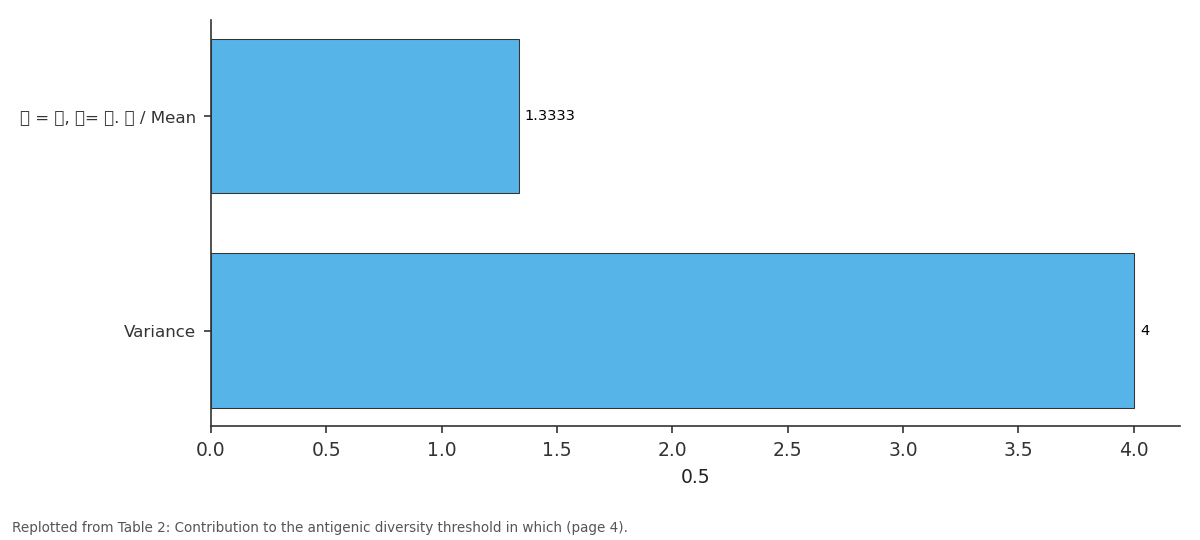
0.5: 𝒂 = 𝟑, 𝜽= 𝟎. 𝟏 / Mean vs Variance
Replotted from Table 2 (page 4) of the original paper. Every bar is the paper's own table value.
View source evidence ↗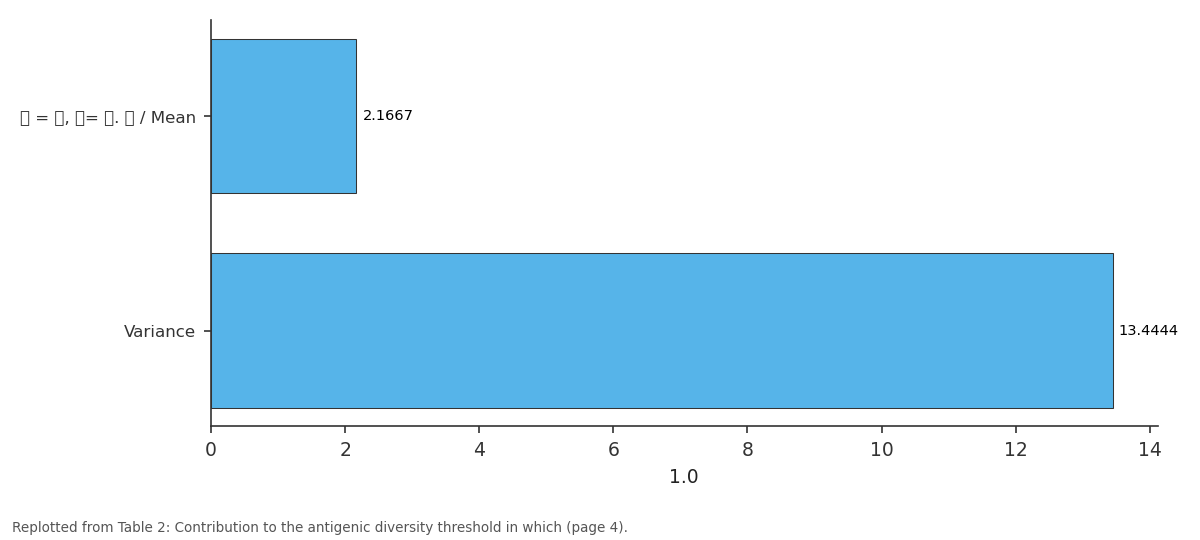
1.0: 𝒂 = 𝟑, 𝜽= 𝟎. 𝟏 / Mean vs Variance
Replotted from Table 2 (page 4) of the original paper. Every bar is the paper's own table value.
View source evidence ↗Figures & tables
From the original paper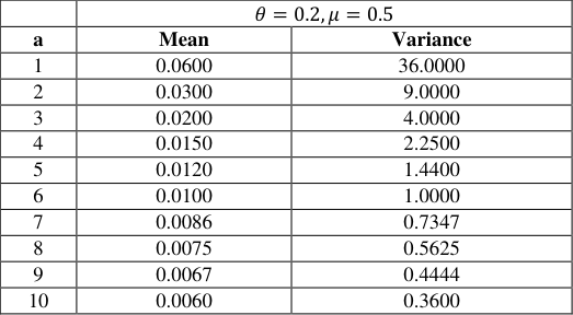 Table 1
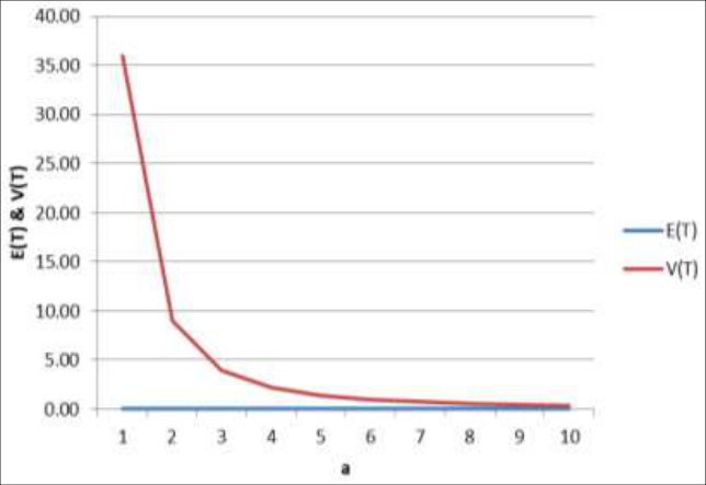 Figure 1
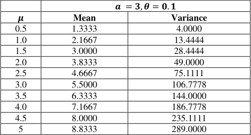 Table 2
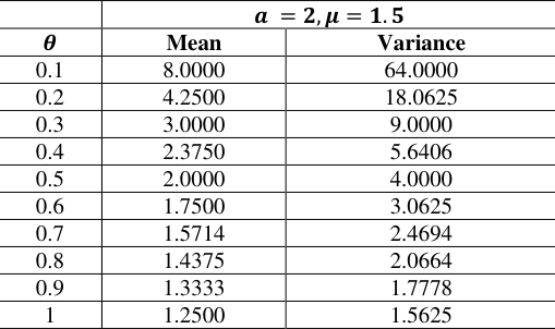 Table 3
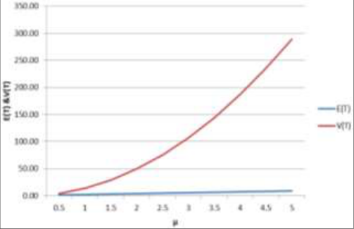 Figure 2
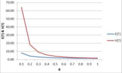 Figure 3
Introduction
The entire world witnessed a pandemic situation with the advent of the terrible and disastrous disease called Acquired Immune Deficiency Syndrome (AIDS) caused by the Human Immunodeficiency Virus (HIV). HIV is a retrovirus, which is RNA-biased and has no DNA. Antigenic diversity is an important determinant of the outcome of HIV infection. Successive invasion through various modes of HIV transmission may contribute to increased HIV antigenic diversity. The idea of the immune system's antigenic variety threshold has been examined by Nowak and May (1991) [3] and Stilianakis et al (1994) [5] . If the overall antigenic diversity produced by HIV exceeds the antigenic diversity threshold, the immune system is unable to defend itself against HIV, which results in immune system collapse and seroconversion occurs rapidly. The probability of transmission through contact is called infectivity. Shiboski and Jewell (1992) [4] obtained the prevalence function expression using available data from partner studies. In the present study, it is assumed that an HIV-uninfected person is infected by an infected person through sexual contact. Every encounter results in the transmission of a small number of HIV particles, which in turn add to the antigenic variety throughout the replication process, which is the regenerative process. The seroconversion occurs when and when the total antigenic diversity reaches a certain level due to the decreasing T 4 Cells. The principles of the cumulative damage process and the shock model served as the foundation for the development of the current model. In Esary et al (1973) [2] , the same was covered in detail. The intercontact times between contacts are considered to be Poisson random variables for the sake of this study. A Generalized Poisson distribution and the uses for it that Anil (2001) [1] mentioned are employed in the creation of the stochastic model. At this point, we assume the following. We view sexual contact as the only source of HIV transmission and assume that a random amount of HIV is transmitted when an uninfected person has sexual contact with an HIVinfected partner. Thus, the individual in this case is subjected to a process of damage acting on the immune system, and the damage is assumed to be nonlinear and cumulative. The transmission of HIV results in harm to persons at each point of contact, and the intervals between encounters are taken to be Poisson random variables. If the total amount of damage surpasses a predetermined limit, which is also subject to random variables. The seroconversion takes place, and the individual is identified as seropositive.
We also assume that the process that creates contacts, the order of damages, and the threshold are independent of one another. We use the symbol Xi to indicate the rise in antigenic diversity brought on by HIV transmission during the ith interaction. Assumed to be continuous random variables are X1, X2,... Let's assume that the antigenic diversity threshold's random variable, Y, has an exponential distribution with parameter. Let G(.) stand for the Xi distribution function and g(.) for the associated p.d.f. The distribution function of the random variable indicating the intervals between subsequent encounters is denoted by the letter F(.). Let gk(.) be the
To denote the Laplace transform of g(x), we will use g*(s). Assume that T represents the period until seroconversion and is a continuous random variable.
Results
Results
S(t) = P(T>t)
= Probability that the seroconversion does not take before t
If we assume that the inter-arrival times between contacts follow an exponential distribution.
Let g(.) follows an exponential distribution with parameter μ
The expected time to seroconversion is given by
Numerical Illustrations
Numerical Illustrations
Conclusion
In table (1), shows the values of statistical measures of seroconversion time corresponding to the variation in 'a' the parameter of the distribution of inter-arrival time when θ and μ are kept fixed. As 'a' increases, the value of a 1 decreases which means the inter-arrival time between contacts becomes smaller and so there is a corresponding decrease in E(T) and V(T). It is observed from the contribution to the antigenic diversity threshold which increases then both E(T) and V(T) increases as indicated in the Table (2) and Fig.
Figures and tables from the paper
| — | 𝜃= 0.2, 𝜇= 0.5 | — |
|---|---|---|
| a | Mean | Variance |
| 1 | 0.0600 | 36.0000 |
| 2 | 0.0300 | 9.0000 |
| 3 | 0.0200 | 4.0000 |
| 4 | 0.0150 | 2.2500 |
| 5 | 0.0120 | 1.4400 |
| 6 | 0.0100 | 1.0000 |
| 7 | 0.0086 | 0.7347 |
| 8 | 0.0075 | 0.5625 |
| 9 | 0.0067 | 0.4444 |
| 10 | 0.0060 | 0.3600 |
Table text extracted from the original PDF; superscript letters are shown inline. The original table image is below.
View original table image
| — | 𝒂 = 𝟑, 𝜽= 𝟎. 𝟏 | — |
|---|---|---|
| 𝝁 | Mean | Variance |
| 0.5 | 1.3333 | 4.0000 |
| 1.0 | 2.1667 | 13.4444 |
| 1.5 | 3.0000 | 28.4444 |
| 2.0 | 3.8333 | 49.0000 |
| 2.5 | 4.6667 | 75.1111 |
| 3.0 | 5.5000 | 106.7778 |
| 3.5 | 6.3333 | 144.0000 |
| 4.0 | 7.1667 | 186.7778 |
| 4.5 | 8.0000 | 235.1111 |
| 5 | 8.8333 | 289.0000 |
Table text extracted from the original PDF; superscript letters are shown inline. The original table image is below.
View original table image
| — | 𝒂 = 𝟐, 𝝁= 𝟏. 𝟓 | — |
|---|---|---|
| 𝜽 | Mean | Variance |
| 0.1 | 8.0000 | 64.0000 |
| 0.2 | 4.2500 | 18.0625 |
| 0.3 | 3.0000 | 9.0000 |
| 0.4 | 2.3750 | 5.6406 |
| 0.5 | 2.0000 | 4.0000 |
| 0.6 | 1.7500 | 3.0625 |
| 0.7 | 1.5714 | 2.4694 |
| 0.8 | 1.4375 | 2.0664 |
| 0.9 | 1.3333 | 1.7778 |
| 1 | 1.2500 | 1.5625 |
Table text extracted from the original PDF; superscript letters are shown inline. The original table image is below.
View original table image
References
5 in the original paper- Anil V. A Generalized Poisson distribution and its applications. Journal of the Kerala Statistical Association. 2001;12:11-22.
- Esary JD, Marshall AW, Proschan F. Shock Model and Wear Processes. The Annals of Probability. 1973;1(4):627-649.
- Nowak MA, May RM. Mathematical Biology of HIV Infection: Antigenic variation and Diversity Threshold. Mathematical Biosciences. 1991;106(1):1-21.
- Shiboski S. Statistical analysis of HIV Infectivity based on the partner studies Biometrics. 1992;46:1133-1150.
- Stilianakis N, Schenzle D, Dietz K. On the antigenic diversity threshold model for AIDS. Mathematical Biosciences. 1994;121(2):235-247.
Cited by 1
From OpenAlex, OpenCitations and reference lists read by Scinovex
- On Estimating the Time from HIV Infection to AIDS - A Stochastic Modeling Approach ↗
R. Jaisankar, S. Deepa · Indian Journal of Science and Technology · 2025
Objectives: To construct a statistical model through which one can estimate the mean time to get AIDS condition in a HIV infected individual. Methods: The methodology adopted for the construction of the statistical model for estimating the time to get AIDS condition considers the antigenic diversity threshold and the antigenic diversity induced by the virus entered through every individual infected…
❝ 0PDF