
Research article · 2023 · Full text
International Journal of Statistics and Applied MathematicsMeasuring value at risk of cryptocurrency using quantum harmonic oscillator
Volume 8(2) · Pages 113–116 · DOI: 10.22271/maths.2023.v8.i2b.966 ↗
Research areasQuantum Computing Algorithms and Architecture
Abstract
Author-writtenCryptocurrency, also known as crypto is a type of digital currency that operates as an exchange mechanism over a computer network and is not supported or maintained by any governing authority. Compared to other equities and bonds, the price of crypto-currencies is highly volatile in nature. Its fluctuations are highly influenced by supply and demand, sentiments of investors and media hype. This paper introduces quantum harmonic oscillator model to measure the value at risk for the fix amount of investment to identify the maximum risk behaviour of cryptocurrency.
Summary
Source-checkedPlain-language reading of the full paper, prepared with AI and checked against the text. Each point links to the authors' own words.
Why it matters
- Cryptocurrencies exhibit high price volatility compared to bonds and other equities, driven by investor sentiment, media hype, and supply and demand. View evidence ↗
- Value at Risk (VaR) is a risk management tool used to estimate potential portfolio losses over a specific timeframe at a certain confidence level. View evidence ↗
The question
- The study aims to use a quantum harmonic oscillator model to measure the Value at Risk (VaR) for a fixed cryptocurrency investment to identify maximum risk behavior. View evidence ↗
What they did
- The researchers used one year of historical Ethereum to Indian currency data from Yahoo Finance, spanning January 1, 2021, to January 1, 2022. View evidence ↗
- The model was applied to a fixed Ethereum investment of 200,000 rupees with a 95% confidence level. View evidence ↗
What they found
- The average return (mean) for the Ethereum data used in the study was 0.021812537. View evidence ↗
- The standard deviation of the quantum harmonic oscillator (QHO) increased as the quantum state increased, ranging from 8.586107942 at state 0 to 25.7583238 at state 4. View evidence ↗
- The study found that Ethereum deviates further from its expected value as the quantum states increase. View evidence ↗
- For the analyzed Ethereum data, the probability distribution function was 0.2139, the probability density function was 0.0458, and the standard deviation was 8.5861. View evidence ↗
- For a hypothetical investment of 200,000 rupees in Ethereum for one week, the expected loss (VaR) at a 95% confidence level was calculated as 27,475.216 (or 27,475.54). View evidence ↗
What it means
- The authors note that calculating VaR using a quantum harmonic oscillator is more complex than classical systems because of intrinsic quantum uncertainties and the difficulty of finding exact solutions. View evidence ↗
Visual summary
1 visualsIllustrations explain the paper; they do not show study data.

Quantum State vs. Volatility
AI-generated conceptual illustration (Quantum harmonic oscillator probability density functions). It explains the idea and does not show study data.
View source evidence ↗Figures & tables
From the original paper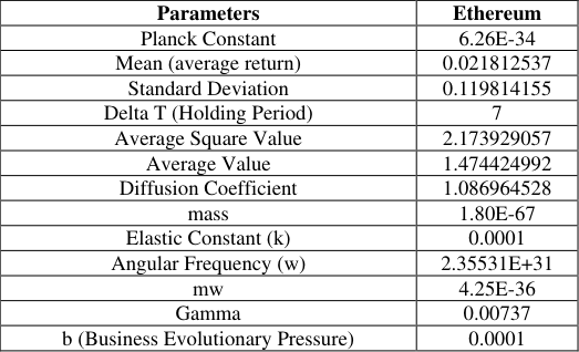 Table 1
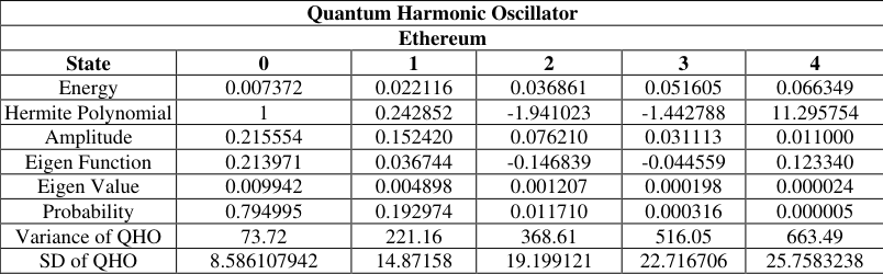 Table 2
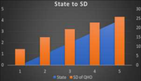 Figure 1
Introduction
It is known that the financial market can be considered risky because it involves the allocation of capital to investments with the potential for both profit and loss. There are several sources of risk in the financial market, including: Market risk: This refers to the risk of changes in market conditions, such as changes in interest rates, currency exchange rates, and equity prices, that can impact the value of financial assets. Credit risk: This refers to the risk of default or creditworthiness of a borrower or issuer of financial instruments, such as bonds. Liquidity risk: This refers to the risk of an inability to buy or sell a financial asset due to a lack of market participants or market depth. Operational risk: This refers to the risk of loss due to operational failures, such as system failures or human error. Political risk: This refers to the risk of loss due to changes in government policies or regulations that can impact the financial market.
These are just a few examples of the many sources of risk in the financial market. The level of risk associated with a particular investment or trade depends on several factors, including the type of asset, the investor's goals, and the market conditions. In summary, the financial market is inherently risky due to the potential for profit and loss, and it is important for investors to understand and manage the risks associated with their investments and trading activities.
To make financial market easily accessible, many different risk management tools are used to get sustainable position in financial market. Risk management tools are critical as they help market participants to identify, assess, and manage risks associated with their investments and trading activities. These methods are used to identify, assess, and control potential losses or uncertainties in financial or business operations. Some of the common risk management tools include: Value at Risk (VaR): provides an estimate of the potential loss that could occur on an investment portfolio over a specified time and with a given level of confidence. Monte Carlo Simulation: uses statistical modelling to simulate various outcomes of a financial decision and estimate the potential losses.
Sensitivity Analysis: assesses the impact of changes in key variables on the outcome of a financial decision. Stress Testing: simulates extreme market scenarios to assess the potential impact on an investment portfolio. Portfolio Diversification: spreading investments across multiple assets to reduce the impact of market risks. Hedging: using financial instruments to reduce the impact of market risks. Insurance: purchasing insurance policies to mitigate potential losses from unforeseen events.
These tools are used by financial institutions, risk managers, and regulators to effectively manage risks and make informed investment decisions. The choice of a particular tool depends on the nature and level of risk involved and the specific needs of the organization.
In this huge range of methods, Value at Risk (VaR) is a widely used risk management tool that provides an estimate of the potential loss that could occur on an investment portfolio over a specified period, with a given level of confidence. It is an essential tool for financial institutions, risk managers, and regulators to measure and manage market risk.
VaR helps investors to make informed investment decisions by providing an assessment of the level of risk involved in a particular investment. The value at risk (VaR) concept can be applied to the quantum harmonic oscillator, which is a fundamental model in quantum mechanics that describes the behaviour of a particle confined in a potential well. In this context, the VaR can be used to assess the risk associated with the uncertainty in the position or momentum of the particle. The calculation of VaR involves estimating the probability distribution of the position or momentum and determining the threshold loss that would not be exceeded with a given level of confidence. The use of VaR in the context of the quantum harmonic oscillator can provide insights into the underlying quantum mechanical principles and help in the development of new quantum-based technologies and applications. However, the calculation of VaR in a quantum mechanical system is more complex than in a classical system, due to the intrinsic quantum mechanical uncertainties and the difficulty in obtaining exact solutions for quantum mechanical problems. Nevertheless, researchers and practitioners are actively exploring new approaches to apply VaR in quantum mechanics, including the use of quantum algorithms and quantum simulation techniques. Calculating Value at Risk (VaR) using a quantum harmonic oscillator involves accounting for the intrinsic quantum mechanical uncertainties. Howev0.er, there are some approaches that can be used to estimate the VaR for a quantum harmonic oscillator mentioned below: Numerical Methods: Numerical methods such as Monte Carlo simulation or finite-difference methods can be used to estimate the VaR for a quantum harmonic oscillator by simulating the position or momentum distributions and calculating the threshold loss that would not be exceeded with a given level of confidence. Analytical Methods: Analytical methods such as the Wigner function or the Husimi function can be used to estimate the position or momentum distribution for the quantum harmonic oscillator. The VaR can then be calculated by determining the threshold loss that would not be exceeded with a given level of confidence. Quantum Algorithms: Quantum algorithms such as quantum Monte Carlo or quantum phase estimation can be used to estimate the position or momentum distributions for the quantum harmonic oscillator. The VaR can then be calculated using the same methods as in numerical or analytical methods.
The choice of method depends on the complexity of the system, the computational resources available, and the level of accuracy required. In general, numerical methods are widely used due to their simplicity and computational efficiency, although they may not always provide an exact solution. Analytical methods and quantum algorithms are more complex but can provide more accurate results.
Literature Review
Goncalves (2013) [4] describes financial volatility risk and its relation to a business cycle-related intrinsic time. This relation was addressed through a multiple round evolutionary quantum game equilibrium which leads to turbulence and multifractal signatures in the financial returns and in the risk dynamics. The model is simulated, and the results are compared with actual financial volatility data. Linsmeier (2000) [7] explain the concept of VAR and then describe in detail the three methods for computing it-historical simulation, the delta-normal method, and Monte Carlo simulation. We also discuss the advantages and disadvantages of the three methods for computing VAR. Finally, we briefly describe stress testing and two alternative measures of market risk.
Ahn et al. (2018) [1] demonstrate that the quantum harmonic oscillator model outperforms traditional stochastic process models, e.g., geometric Brownian motion and the Heston model, with smaller fitting errors and better goodness of fit statistics. The solution of the Schrodinger equation for the quantum harmonic oscillator shows that stock returns follow a mixed distribution, which describes Gaussian and non-Gaussian features of the stock return distribution. In addition, they provide an economic rationale of the physics concepts such as the eigenstate, eigenenergy, and angular frequency, which sheds light on the relationship between finance and Physics literature. Jeknić-Dugić (2018) [5] pursued the quantum-mechanical challenge to the efficient market hypothesis for the stock market by employing the quantum Brownian motion model. He also introduced the external harmonic field for the Brownian particle and use the quantum Caldeira-Leggett master equation as a potential phenomenological model for the stock market price fluctuations. Lee et al. (2020) [6] examined the weak-form efficient market hypothesis of the crude palm oil market by adopting the quantum harmonic oscillator. This method permits Lee to analyse market efficiency by approximating one constraint: the probability of finding the market in a ground state where conclusion established that the crude palm oil market is more efficient than the West Texas Intermediate crude oil market. Orrell (2020) [9] addressed issues regarding intrinsically uncertain demand by consuming a quantum context to model supply and demand as, not a cross, but a probabilistic wave, with an allied entropic force. The approach is used to derive from first principles a technique for modelling asset price changes using a quantum harmonic oscillator that has been previously used and empirically tested in quantum finance. The method is established for a simple system and claims in other areas of economics are discussed. Ryu (2021) [10] looked at the weak-form efficient market theory because the log price series for REIT stocks for US REIT equities, contradicted the random walk theory as a model specification, the variance ratio test revealed that the general stock market and REIT markets were not efficient in the weak-form. Instead, he used the quantum harmonic oscillator to present definite evidence. The ground state solution for a random walk included in the quantum harmonic oscillator turned out to be a more effective way to test the efficient market hypothesis. Bhatt and Gor (2022) [2] showcased an interesting structure of Risk Neutral system. They also examine single step and multistep quantum binomial option pricing model. This approach elaborates circuit proposed by A. Meyer. Bhatt and Gor (2022) [3] review applications of quantum harmonic oscillator model in financial mathematics and discussed about different applications of quantum harmonic oscillator and its characteristics. Zhang (2022) [11] enhances the IOAS algorithm's neighbourhood and out-of-bounds movement rules. It then suggests the DETS support vector regression algorithm, which is based on enhanced tabu search and differential evolution and uses error indicators to compare related algorithms. The findings demonstrate the algorithm's effectiveness and viability in exchange rate prediction. Mba, (2022) [8] examined the typical mean-variance (MV) optimization model in this work by means of two modifications to the MV formulation. Additionally, these results demonstrate that equities with lower behavioural scores do better than counterpart portfolios with higher behavioural scores.
Methodology and Data Collection
In this paper, historical data of Ethereum is collected from YAHOO Finance website. Historical data for the Ethereum to Indian currency is collected here in the time span of one year from 1 st January 2021 to 1 st January 2022. Calculating Value at Risk for a quantum harmonic oscillator involves estimating the probability distribution of the position or momentum and determining the threshold loss that would not be exceeded with a given level of confidence. Here's an example of how to calculate Value at Risk for the position of a quantum harmonic oscillator using a numerical method.
Assuming that the position of the particle in the quantum harmonic oscillator is described by the Hamiltonian
, where 𝑝 is the momentum operator, 𝑚 is the mass of the particle, and 𝜔 is the frequency of the oscillator. Monte Carlo simulation can be used to estimate the position distribution and to calculate the Value at Risk. Descriptive analysis of the Ethereum is provided in the table mentioned below: As the Fick's First Law states, flux is proportional to the concentration gradient, and the proportionality constant D is the diffusion coefficient. Diffusion coefficient is the ratio of flux density to the negative of the concentration gradient in direction of diffusion. Here different physical entities of the Ethereum are mentioned in below table for different states.
Variance of the quantum harmonic oscillator is given by:
Moreover, the time evolution of the probability density function (PDF) refers to how the PDF changes over time for a given stochastic system. The PDF represents the distribution of a set of random variables and its time evolution can be described by mathematical models, such as the Fokker-Planck equation or other partial differential equations. Here probability distribution function can be calculated by the eigenfunction developed by the model. Below table showcases different values for respective states of Ethereum: exceeded with a given level of confidence, for example, 95%. The threshold loss can be calculated as 𝑥 -𝑍𝜎, where Z is the z-score corresponding to the given level of confidence. Step 4: The Value at Risk is the maximum loss that can be expected with a given level of confidence, which is equal to the threshold loss in this case:
The actual calculation of value at risk depends on the specific system, the wave function and the level of confidence interval. These steps are used to find VaR of Ethereum for fixed investment of rupees 2,00,000/-with 95% level of confidence.
Results
Let the investment is fixed for rupees 2,00,000/-in Ethereum and as the probability distribution function and probability density function for the quantum harmonic oscillator is given as:
) and ᴪ(𝑥) ( Here value at risk is found to be 27475.216.
Here hypothetical situation of Investing Rs. 2,00,000 for 1 Week in Ethereum gives expected loss of 27,475.54 with 95% Confidence Level.
Graphical Representation
Graphical Representation
Conclusion
This paper proposes quantum harmonic oscillator to find the Value at Risk (VaR) for cryptocurrency. However, calculating VaR for a quantum harmonic oscillator is more complex than in a classical system due to the intrinsic quantum mechanical uncertainties and the difficulty in obtaining exact solutions. The approach involves generating random samples of the position or momentum, calculating the expected value and standard deviation, and determining the threshold loss. The Monte Carlo method provides an efficient and flexible way to estimate VaR in the context of quantum harmonic oscillators, as it can be adapted to different systems, wave functions, and levels of confidence. Overall, the application of Monte Carlo method to the quantum harmonic oscillator can provide valuable insights into the underlying quantum mechanical principles and contribute to the development of new quantumbased technologies and applications.
Figures and tables from the paper
| Parameters | Ethereum |
|---|---|
| Planck Constant | 6.26E-34 |
| Mean (average return) | 0.021812537 |
| Standard Deviation | 0.119814155 |
| Delta T (Holding Period) | 7 |
| Average Square Value | 2.173929057 |
| Average Value | 1.474424992 |
| Diffusion Coefficient | 1.086964528 |
| mass | 1.80E-67 |
| Elastic Constant (k) | 0.0001 |
| Angular Frequency (w) | 2.35531E+31 |
| mw | 4.25E-36 |
| Gamma | 0.00737 |
| b (Business Evolutionary Pressure) | 0.0001 |
Table text extracted from the original PDF; superscript letters are shown inline. The original table image is below.
View original table image
| Quantum Harmonic Oscillator | — | — | — | — | — |
|---|---|---|---|---|---|
| Ethereum | |||||
| State | 0 | 1 | 2 | 3 | 4 |
| Energy | 0.007372 | 0.022116 | 0.036861 | 0.051605 | 0.066349 |
| Hermite Polynomial | 1 | 0.242852 | -1.941023 | -1.442788 | 11.295754 |
| Amplitude | 0.215554 | 0.152420 | 0.076210 | 0.031113 | 0.011000 |
| Eigen Function | 0.213971 | 0.036744 | -0.146839 | -0.044559 | 0.123340 |
| Eigen Value | 0.009942 | 0.004898 | 0.001207 | 0.000198 | 0.000024 |
| Probability | 0.794995 | 0.192974 | 0.011710 | 0.000316 | 0.000005 |
| Variance of QHO | 73.72 | 221.16 | 368.61 | 516.05 | 663.49 |
| SD of QHO | 8.586107942 | 14.87158 | 19.199121 | 22.716706 | 25.7583238 |
Table text extracted from the original PDF; superscript letters are shown inline. The original table image is below.
View original table image
References
11 in the original paper- Ahn K, Choi M, Dai B, Sohn S, Yang B. Modelling stock return distributions with a quantum harmonic oscillator. EPL (Europhysics Letters). 2018;120(3):38003.
- Bhatt A, Gor R. Examining Single step and Multistep Quantum Binomial Option Pricing Model. IOSR Journal of Economics and Finance (IOSR-JEF). 2022;13(3):5260.
- Bhatt A, Gor R. A Review paper on Quantum harmonic oscillator and its applications in finance. IOSR Journal of Economics and Finance (IOSR-JEF). 2022;13(3):61-65.
- Gonçalves CP. Quantum financial economics-risk and returns. Journal of Systems Science and Complexity. 2013;26(2):187-200.
- Jeknić-Dugić J, Petrović I, Arsenijević M, Dugić M. Quantum Brownian oscillator for the stock market. arXiv preprint arXiv: 1901.10544; c2018
- Lee GH, Joo K, Ahn K. Market efficiency of the crude palm oil: Evidence from quantum harmonic oscillator. In Journal of Physics: Conference Series. 2020 1593(1):012037).
- Linsmeier TJ, Pearson ND. Value at risk. Financial Analysts Journal. 2000;56(2):47-67.
- Mba JC, Ababio KA, Agyei SK. Markowitz MeanVariance Portfolio Selection and Optimization under a Behavioural Spectacle: New Empirical Evidence. International Journal of Financial Studies. 2022;10(2):28.
- Orrell D. A quantum model of supply and demand. Physica A: statistical Mechanics and its Applications. 2020;539(1):122928.
- Ryu I, Jang H, Kim D, Ahn K. Market efficiency of US REITs: A revisit. Chaos, Solitons & Fractals. 2021;150:111070.
- Zhang X, Zhong C, Abualigah L. Foreign exchange forecasting and portfolio optimization strategy based on hybrid-molecular differential evolution algorithms. Soft Computing. 2023;27(7):3921-3939.