
Research article · 2023 · Full text
International Journal of Geography Geology and EnvironmentClimatological impact on groundnut crop over Junagadh district
Volume 5(1) · Pages 57–66 · DOI: 10.22271/27067483.2023.v5.i1a.142 ↗
Research areasClimate change impacts on agricultureClimate variability and modelsPeanut Plant Research Studies
Abstract
Author-writtenThe present study investigated the climatic vulnerability of the peanut cropping system in Gujarat's Junagadh district. The Junagadh district is situated in western Gujarat between the latitudes of 70.150 and 70.550 and the longitudes of 20.470 and 21.450. One of the significant oil seed crops in India is the groundnut crop. Gujarat is India's top groundnut producer. Gujarat's Junagadh district produces the majority of the state's ground net crops. Planning for climate change mitigation efforts requires an understanding of the past, present, and projected temperatures and precipitation in the Junagadh district. IMD provided historical daily temperature data with a resolution of 100 km for the years 1951 to 2019.Historical daily temperature data from 1951 to 2019 is downscaled to 1 km from IMD at a resolution of 100 km x 100 km. Data on historical precipitation was downscale from Cru's 25 km x 25 km resolution to 10 km. The temperature projections (RCP 4.5 and RCP 8.5) for five South Asian codex domain models at resolutions of 50 km x 50 km and scaled down to 1 km are displayed. 50 km x 50km and 10km downscale daily data from five South Asian codex domain models. The Taylor diagram demonstrated that, when tested against cru data, all models perform better in terms of rainfall and temperature. The cm5a model outperformed the other models in terms of performance. Maximum temperatures are seen to rise from 32.760 C to 35.50 C (RCP 4.5) and 37.20 C (RCP 8.5) and minimum temperatures are seen to rise from 23.920 C to 25.300 C (RCP 4.5) and 27.480 C between 1970 and 2100 (RCP 8.5). June, a crucial month for the germination stage of groundnut crops, sees an increase in both the maximum and minimum temperatures. From 1970 to 2100, June to November total precipitation increased from 853.2 mm to 1029 (RCP 4.5) and 1097 mm, respectively (RCP 8.5).
Summary
Source-checkedPlain-language reading of the full paper, prepared with AI and checked against the text. Each point links to the authors' own words.
Why it matters
- Groundnut is a critical oilseed crop in India, with Gujarat being the leading producer and the Junagadh district contributing the majority of the state's output. View evidence ↗
- In many tropical regions, crops are approaching their heat tolerance limits, which threatens to reduce overall yields. View evidence ↗
- Crop production is significantly impacted by biophysical changes caused by rising temperatures, changing rainfall patterns, and increased atmospheric carbon dioxide. View evidence ↗
The question
- The study aimed to investigate how vulnerable the peanut cropping system in the Junagadh district of Gujarat is to climatic changes. View evidence ↗
What they did
- The researchers used historical temperature data (1951–2019) from the IMD, downscaled to 1 km, and precipitation data from CRU, downscaled to 10 km. View evidence ↗
- Future temperature projections were analyzed using five South Asian CORDEX domain models under RCP 4.5 and RCP 8.5 scenarios, downscaled to 1 km. View evidence ↗
- The analysis employed linear regression for trend detection and calculated spatial standard deviation, variance, and various time-based averages. View evidence ↗
What they found
- Between 1970 and 2100, maximum temperatures are projected to rise from 32.76°C to 35.50°C (RCP 4.5) or 37.20°C (RCP 8.5), while minimums are projected to rise from 23.92°C to 25.30°C (RCP 4.5) or 27.48°C (RCP 8.5). View evidence ↗
- Total precipitation from June to November is projected to increase from 853.2 mm to 1029 mm under RCP 4.5 and 1097 mm under RCP 8.5 between 1970 and 2100. View evidence ↗
- Multi-variant analysis showed that combined climate parameters could explain up to 39% and 30% of the variation in groundnut yield. View evidence ↗
What it means
- The authors conclude that groundnut yield is directly proportional to precipitation, whereas no significant relationship was found between temperature and yield. View evidence ↗
- The authors predict that future groundnut crop yields will increase as precipitation increases. View evidence ↗
Visual summary
1 visualsIllustrations explain the paper; charts are replotted from the paper's own table values.
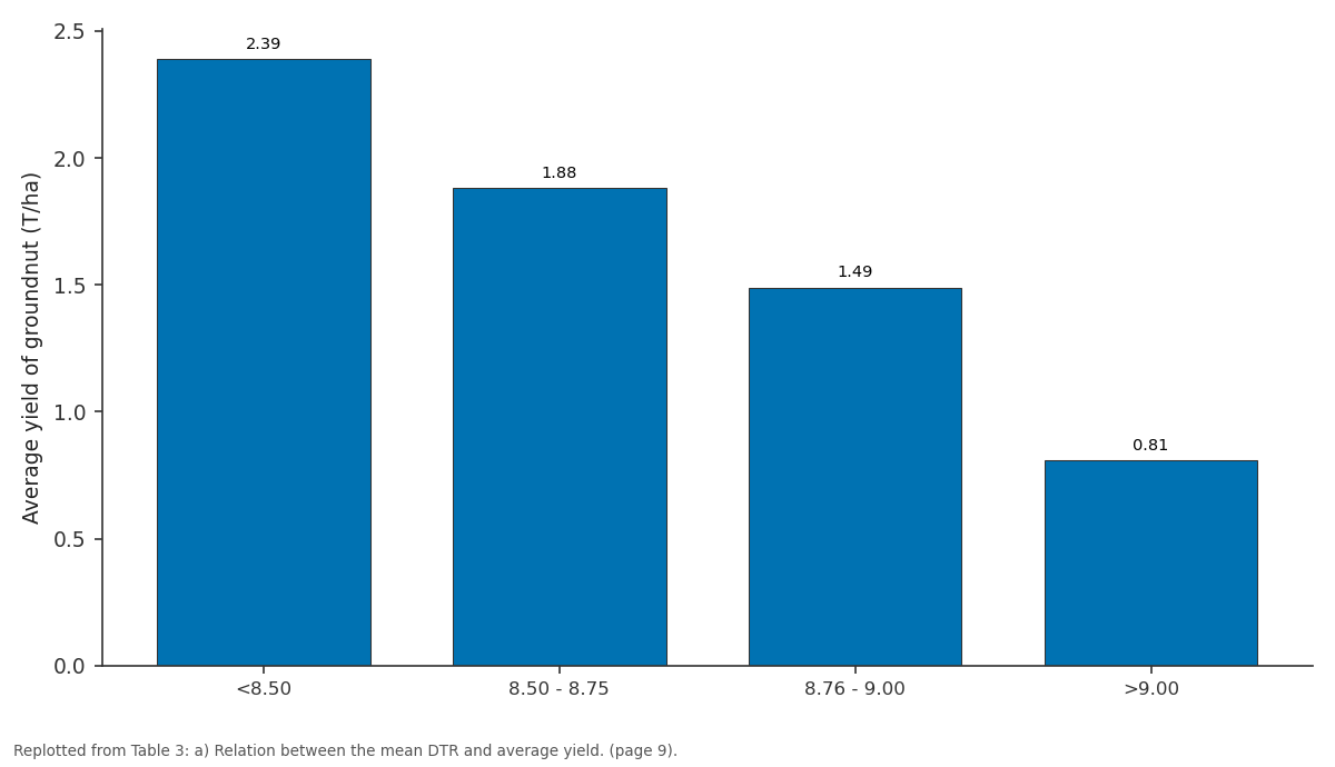
Average yield of groundnut (T/ha): <8.50 vs 8.50 - 8.75 vs 8.76 - 9.00 vs >9.00
Replotted from Table 3 (page 9) of the original paper. Every bar is the paper's own table value.
View source evidence ↗Figures & tables
From the original paper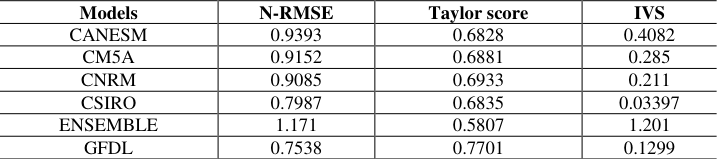 Table 1Page 4
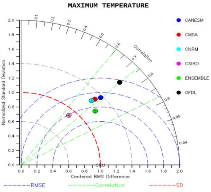 Figure 1Page 4
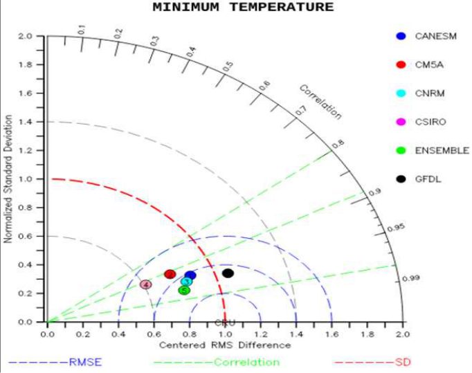 Figure 1Page 4
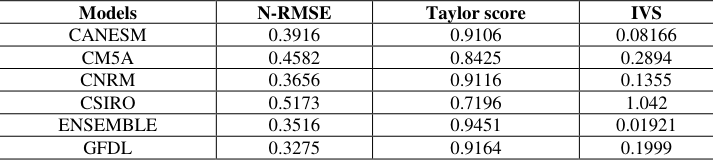 Table 1Page 5
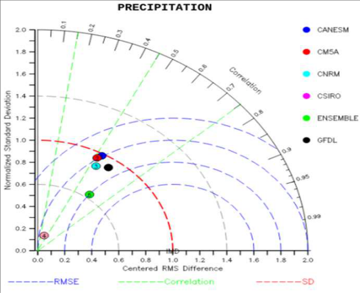 Figure 1Page 5
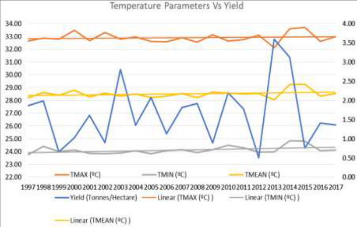 Figure 2Page 5
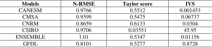 Table 1Page 6
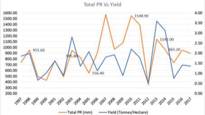 Figure 3Page 6
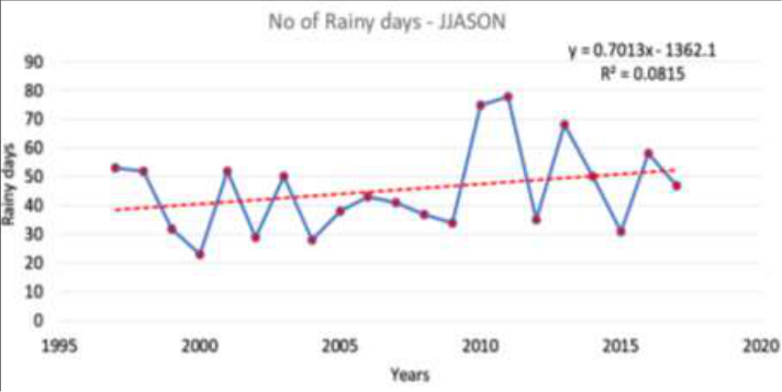 Figure 4Page 6
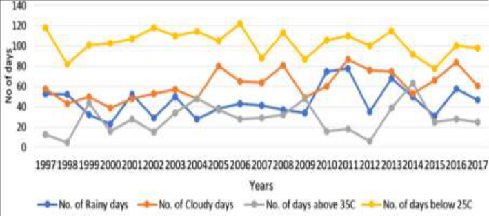 Figure 5Page 6
 Table 2Page 7
 Table 2Page 7
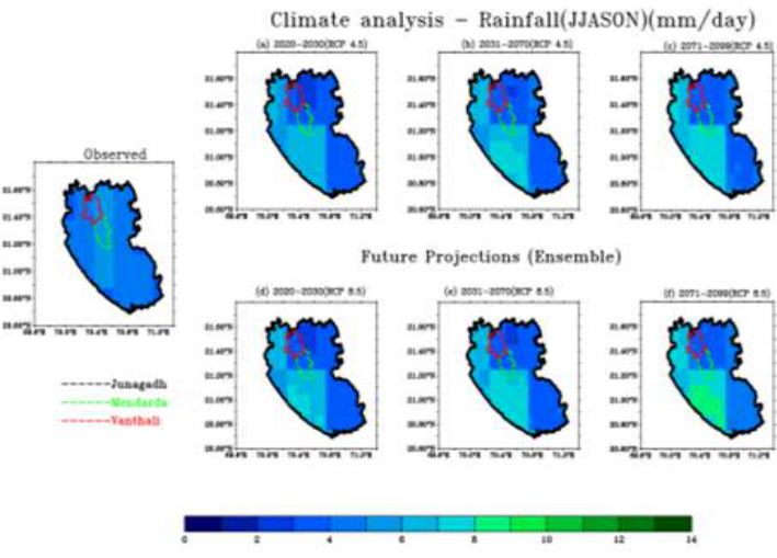 Figure 6Page 7
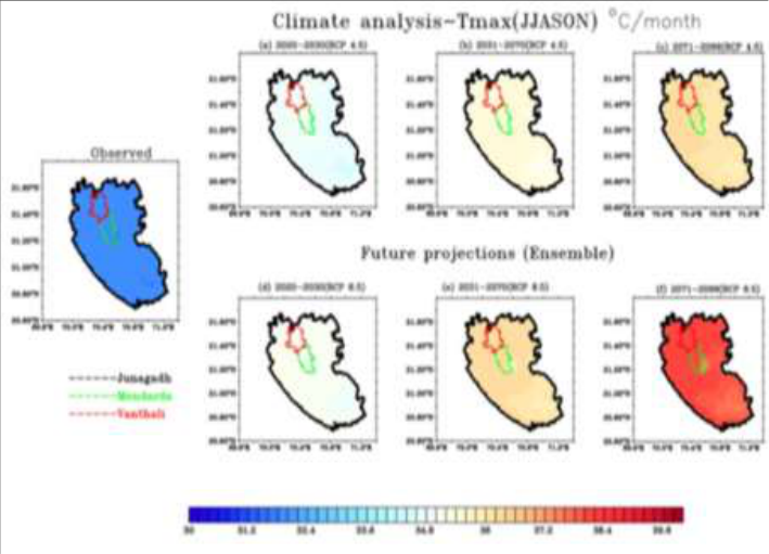 Figure 6Page 7
 Table 2Page 8
 Table 2Page 8
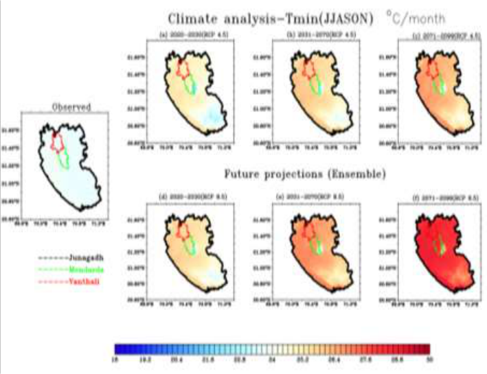 Figure 6Page 8
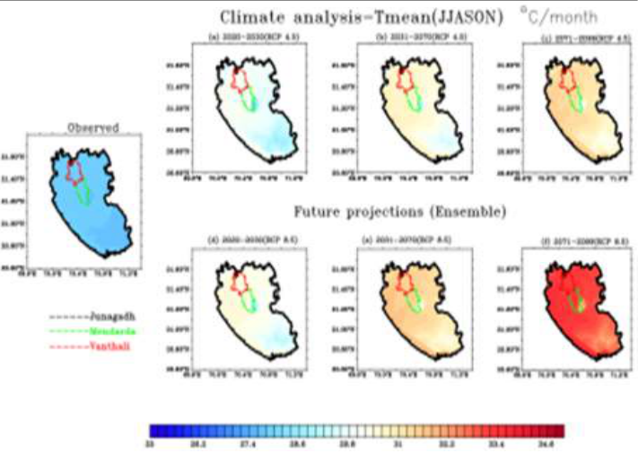 Figure 6Page 8
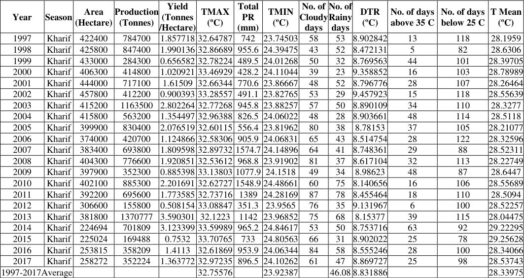 Table 3Page 9
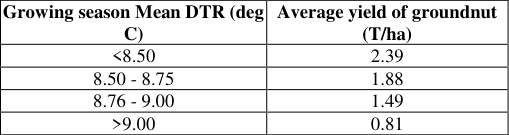 Table 3Page 9
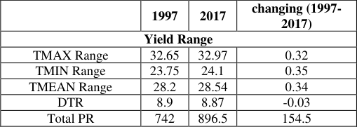 Table 3Page 9
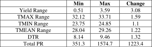 Table 3Page 9
 Table 3Page 9
 Table 3Page 9
Introduction
The important grain legume crop known as groundnut is grown primarily for its use as a source of vegetable protein and edible oil. The production of peanuts takes place in the tropical and semi-arid tropical regions, which are characterized by high temperatures and little rainfall, to the tune of about 90% of the global total. In the majority of tropical regions, crops are getting close to the point where they can tolerate no more heat, which could result in lower crop yields. The ideal air temperature for groundnut terminative growth is between 260 and 300 °C, which is higher than the ideal air temperature for reproductive growth, which is between 220 and 250 °C (Cox, 1991) [11] . Meteorological factors, such as rising temperatures, shifting precipitation patterns, and rising atmospheric carbon dioxide levels, have a significant biophysical impact on crop production (H.R. Patel et al., 2013) [8] . The biophysical effects of climate change on agricultural production will vary over time and will be positive or negative depending on the type of agricultural system and region. Gujarat, Andhra Pradesh, Tamil Nadu, Karnataka, and Maharashtra account for 80 percent of India's land area and 84 percent of its production. Gujarat leads all of them in terms of both production and area (forest report, Directorate of agriculture, Gujarat state). In Gujarat, groundnut productivity averages 1603 kg/ha during the Kharif season and 1903 kg/ha during the summer (Anonymous, 2012b). The average global temperature had risen 1.80 °C by 2100, reaching 40 °C (IPCC, 2014).In addition to the increase in temperature, the frequency of extreme weather events such as heat waves, floods, cyclones, and droughts is expected to rise. These parameters are bound to have an impact on agricultural production.
Temperature increases of 10 °C to 30 °C may cause a reduction in groundnut production (24%), as has been reported with temperature increases of 2.80 °C to 7.70 °C (Patel et al., 2008) [12] . When the maximum temperature was raised by 30 degrees Celsius, pod yield decreased by 39 to 48 percent in different cultivars, with the minimum temperature having less of an effect than the maximum temperature (B.M. Mote, 2016) [3] . In comparison to other food crops, the mean temperature varied with crop production.
Data
The India Meteorological Department, Government of India (Pai et al. 2014) [13] and the Climate Research Unit (CRU) of East Anglia, UK (Harris et al. 2014) [14] provide observed gridded climatology data for temperature and rainfall. Temperature data is further downscaled to 1 km resolution by adjusting temperatures in relation to a high-resolution digital elevation model (Gerlitz et al. 2014, Farr et al. 2007, and Reuter et al. 2007) [15][16][17] . IMD's gridded rainfall data has a much finer spatial resolution, i.e., 0.25° x 0.25°. (Pai et al., 2014) [13] . This high resolution observed rainfall dataset (1901-2015) is downscaled further using NASA's GPM precipitation data, which is available at a resolution of 10 km from 2003 to 2019. This downscaled data is used to analyse rainfall profiles and trends in the study area, as well as to correct for bias in future temperature and rainfall projections in the study area. Future projections for four Representative Concentration Pathways (RCP) scenarios are provided in global climate models. In this study, we used the RCP scenarios RCP4.5 and RCP8.5. RCP 2.6, RCP 4.5, RCP 6.0, and RCP 8.5 are the four RCP scenarios. These scenarios are written in such a way that they cover the entire spectrum of stabilization, mitigation, and baseline emission scenarios available in the literature. The naming convention reflects socioeconomic pathways that will reach a specific radiative forcing by 2100. RCP 8.5, for example, results in a radiative forcing of 8.5 Wm-2 by 2100. While there are four RCP scenarios available, we have used RCP4. 5
Methodology
The observed data for temperature (Tmax, Tmin) was of coarse resolution. We needed high-resolution data as the study area was small. For this purpose, we interpolated the existing observed data using the bilinear method and brought it down to 1 km x 1 km resolution. For precipitation data, we implemented CNN by taking the satellite data and IMD data and producing a merged dataset that was of 10 km x 10 km resolution. In the present study, we have taken five CORDEX models for the South Asian domain (WAS-44). As the resolutions of each model were different and the study area was small, we interpolated the model data to a 1 km x 1 km resolution for Tmax and Tmin using the bilinear method. For precipitation, we interpolated it to a 10 km x 10 km resolution. Tmax and Tmin datasets were further subjected to lapse rate correction to bring out the local features of the area. Tmean was computed using Tmax and Tmin. All the datasets were spatially averaged for the Junagadh, Vanthali, and Mendarda regions separately. Trend analysis has been done using the linear regression method. The standard deviation and variance were calculated spatially for each time step. Monthly, yearly, and decadal averages were computed for both observed and model datasets. An ensemble mean of all the model datasets has been computed. Bias correction has been done on model datasets. The bias computed in the historical data (Observed, model) was added to the future projections. The models were subjected to different skill tests to determine the best among them. Taylor's diagram has been plotted for Tmax, Tmin, Tmean, and precipitation. The Taylor scores, Root Mean Square Error (RMSE), and Interannual Variability skill score (IVS) have been computed.
Results and Discussion
In the present study, we studied the climatological impact of the meteorological parameters such as rainfall, maximum and minimum temperatures on the ground net crop in Junagadh district. We have conducted experiments using ensemble models of future projections of the two climate scenarios, RCP 4.5 and RCP 8.5. The results are presented here. The future projections are studied over a period of 100 years, i.e., up to 2100. Three major time periods have been studied for both the scenarios: time period one (2020-2030), time period two (2030-2070), and time period three (2070-2100). Monthly wise climate analysis was done for the parameters of rainfall, maximum, and minimum temperature of the months of June, July, August, September, October, and November, which are the most prominent months for the growth and yield of the ground net crop. A figure 2 depicts the comparison of the maximum, minimum, and means temperatures and yield over the Junagadh District from 1971 to 2017. As the temperature rises over time, the yield production declines in both the maximum and minimum temperatures. The mean or optimum temperature is critical for crop productivity. Figure 3 depicts total precipitation and yield across the Junagadh district from 1971 to 2021. The graph illustrates that rainfall is an important determinant for groundnut yield production; when rainfall is high, so is production; there is a direct relationship between yield and rainfall. Figure 4 shows the number of rainy days and Figure 5 depicts a comparison between the number of cloudy days, rainy days, and the maximum temperature of 35 degrees Celsius and the minimum temperature of 25 degrees Celsius. As the number of cloudy days and rainy days increase, so does the temperature, and the lower level moisture increases, creating a flood condition that may be favorable to ground nuts? As the number of cloudy days increases, so does the yield quality and output. And while to better understand microclimatological phenomena and their effects on crops, the district has been divided into three major blocks: Junagadh, Mendarda, and Vanthali. Figure 6 (a) shows the climate analysis of rainfall for the JJASON month using an ensemble of models for the three time series of the two scenarios and comparing it to the Junagadh district's climatologically mean rainfall (1971-2019). The average climatologically measured rainfall in Junagadh village for the JJASON month is 4.7 mm/day, with a maximum of 5.8 mm/day and a minimum of 3.6 mm/day, as shown in fig 6(a).The model forecasted average rainfall. The model ensembles in RCP 4.5, on the other hand, show a maximum of 7.1 mm per day, which is 0.9 percent higher than the mean rainfall.
Analysis of the maximum temperature for JJASON Fig. 6 (b): Climate analysis for the JJASON month using an ensemble of models for the three time series of the two scenarios and compared to the Junagadh district's climatologically mean maximum temperature (1971-2019). The mean climatological maximum temperature for the JJASON month in Junagadh village is 32 °C/day, as shown in fig. 6 (b). The model indicates that the average maximum temperature will be in RCP 4.5, however, the model ensembles show a maximum of 38 °C each day. In the second time period (2031-2070), the average temperature rises to 34.2 0 degrees Celsius, with a maximum of 39.10 0 Celsius and a minimum of 29.3 0 Celsius every day. In the decade (2071-2099), 36.10 0 Celsius with a maximum of 31.2-41 0 Celsius each day, in contrast to RCP 8.5. In both circumstances, the maximum temperature rises.
Analysis of the minimum temperature for JJASON
Analysis of the minimum temperature for JJASON
Analysis of the mean temperature for JJASON
Temperature is more significant than rainfall for crop development and productivity. Growth and development require optimal temperatures. In this study, we looked at the maximum and minimum temperature differences during the last three decades for both scenarios, from June to November. The climatological maximum temperature for June in the Junagadh district is 33 0 degrees Celsius. Fig. 6 (d): Climate analysis for the JJASON month using an ensemble of models for the three time series of the two scenarios and compared to the Junagadh district's climatologically mean temperature (1971-2019). The mean climatological temperature for the JJASON month in Junagadh village is 27.8 °C/day, as shown in fig. 6(d).The model anticipated the average temperature at In RCP 4.5, the model ensembles suggest a maximum of 26.50c each day. The average temperature rises to 28.9 0 Celsius in the second time period (2031-2070), with a maximum of 330 degrees Celsius and a minimum of 25.9 0 Celsius every day. In the decade (2071-2099), 29.5 °C with a maximum of 27.7-35.4 °C/day compared to RCP 8.5.
Regression Analysis (yield) (Table-3 (d))
The relationship between climate elements and the yield is analyzed through correlation with the null hypothesis (Ho) that there is a significant correlation in temperature (0.40) and precipitation (0.48). Regarding rainfall, temperature, and groundnut, the correlation coefficient of 0.48 and 0.40 is interpreted as a strong positive relationship between the two variables. The significance 2-tailed gives a P value of 0.06, which is greater than 0.05. Hence, the Ho is retained. The study does not provide enough evidence to conclude that there is a statistically significant correlation between temperature and ground nut yield. In terms of regression, HO is that there is no supported relationship between temperature and groundnut yield (b=0). The results give an R value of 0.4 and an R square of 0.16, meaning temperature explains only 16% of the ground nut yield. The significance 2-tailed gives a P value of 0.02, which is less than 0.05. Hence, H0 is rejected and Ha is accepted, suggesting that a unit increase in rainfall results in a unit increase in the yield of groundnut. The regression analysis indicates an R value of 0.23 and an R square of 0.23 explains 23% of the ground nut yield.
Analysis of multiple regression (Table-3(e))
In this Multi-variant Analysis of Max-Temperature, Min-Temperature, Rainy Days, Cloudy Days, and Groundnut, yield is taken as the independent variable and pairs of (Temperature, Rainy Days), (Temperature, Precipitation, Rainy Days), (Temperature, Precipitation, Rainy Days), (Temperature, Precipitation, Rainy Days), (Temperature, Precipitation, Rainy Days), (Temperature, Precipitation, Rainy Days), (Temperature, Precipitation, Rainy Days), (Temperature, Precipitation, Rainy Days), (Temperature, Precipitation, Rainy Days), (Temperature, Precipitation, Rainy Days The significance level at 2-tailed is 0.03 and 0.03, which is less than 0.05. Hence, Ho is rejected. The regression analysis indicates R values of 0.63 and 0.55 and R squares of 0.39 and 0.3, suggesting that accounts for 39% and 30% of the variation in ground nut yield. The correlation coefficients for (Temperature, precipitation); (Temperature, precipitation, rainy days); and (Temperature, cloudy, rainy days) are 0.59, 0.62, and 0.59, respectively. The significance 2-tailed is 0.06, 0.07, and 0.12, which is greater than 0.05. Hence, Ho is retained. The regression analysis indicates an R value of 0.59, 0.62, 0.59 and an R square of 0.35, 0.39, and 0.35, suggesting that accounts for 35%, 39%, and 35% of the variation in ground nut yield. Celsius, and 12.78 0 Celsius, respectively. Precipitation and temperature are increasing in the RCP (4.5 and 8.5) future period compared to observed data. The association between the met parameters and groundnut crop yield can be identified here. We can see from this relationship that precipitation and yield have a correlation of 0.48 and a significance of 0.02. As a result, yield will increase with precipitation and vice versa. The correlation between maximum temperature and yield is 0.42, with a significance of 0.06. As a result, we can conclude that there is no linear relationship between these two variables. In my investigation, yielding was shown to be directly proportionate to precipitation, with no significant found between temperatures and yielding.
Figures and tables from the paper
| Models | N-RMSE | Taylor score | IVS |
|---|---|---|---|
| CANESM | 0.9393 | 0.6828 | 0.4082 |
| CM5A | 0.9152 | 0.6881 | 0.285 |
| CNRM | 0.9085 | 0.6933 | 0.211 |
| CSIRO | 0.7987 | 0.6835 | 0.03397 |
| ENSEMBLE | 1.171 | 0.5807 | 1.201 |
| GFDL | 0.7538 | 0.7701 | 0.1299 |
Table text extracted from the original PDF; superscript letters are shown inline. The original table image is below.
View original table image
| Models | N-RMSE | Taylor score | IVS |
|---|---|---|---|
| CANESM | 0.3916 | 0.9106 | 0.08166 |
| CM5A | 0.4582 | 0.8425 | 0.2894 |
| CNRM | 0.3656 | 0.9116 | 0.1355 |
| CSIRO | 0.5173 | 0.7196 | 1.042 |
| ENSEMBLE | 0.3516 | 0.9451 | 0.01921 |
| GFDL | 0.3275 | 0.9164 | 0.1999 |
Table text extracted from the original PDF; superscript letters are shown inline. The original table image is below.
View original table image
| Models | N-RMSE | Taylor score | IVS |
|---|---|---|---|
| CANESM | 0.9766 | 0.5512 | 0.001453 |
| CMSA | 0.9399 | 0.5475 | 0.06737 |
| CNRM | 0.8659 | 0.6133 | 0.0304 |
| CSIRO | 0.9706 | 0.03551 | 45.95 |
| ENSEMBLE | 1.01 | 0.5347 | 0.01156 |
| GFDL | 0.8101 | 0.5277 | 0.8728 |
Table text extracted from the original PDF; superscript letters are shown inline. The original table image is below.
View original table image
| Year | Season | Area (Hectare) | Production (Tonnes) | Yield (Tonnes /Hectare) | TMAX (ºC) | Total PR (mm) | TMIN (ºC) | No. of Cloudy days | No. of Rainy days | DTR (ºC) | No. of days above 35 C | No. of days below 25 C | T Mean (ºC) |
|---|---|---|---|---|---|---|---|---|---|---|---|---|---|
| 1997 | Kharif | 422400 | 784700 | 1.857718 | 32.64787 | 742 | 23.74503 | 58 | 53 | 8.902842 | 13 | 118 | 28.1959 |
| 1998 | Kharif | 425800 | 847400 | 1.990136 | 32.86689 | 955.6 | 24.39475 | 43 | 52 | 8.472131 | 5 | 82 | 28.6306 |
| 1999 | Kharif | 433000 | 284300 | 0.656582 | 32.78224 | 489.5 | 24.01268 | 50 | 32 | 8.769563 | 44 | 101 | 28.39705 |
| 2000 | Kharif | 406300 | 414800 | 1.020921 | 33.46929 | 428.2 | 24.11044 | 39 | 23 | 9.358852 | 16 | 103 | 28.78989 |
| 2001 | Kharif | 444000 | 717100 | 1.61509 | 32.66344 | 770.6 | 23.86667 | 48 | 52 | 8.796776 | 28 | 107 | 28.26464 |
| 2002 | Kharif | 457800 | 412200 | 0.900393 | 33.28557 | 491.1 | 23.82765 | 53 | 29 | 9.457923 | 15 | 118 | 28.55639 |
| 2003 | Kharif | 415200 | 1163500 | 2.802264 | 32.77268 | 945.8 | 23.88257 | 57 | 50 | 8.890109 | 34 | 110 | 28.3277 |
| 2004 | Kharif | 415800 | 563200 | 1.354497 | 32.96388 | 826.5 | 24.06022 | 48 | 28 | 8.903661 | 48 | 114 | 28.5118 |
| 2005 | Kharif | 399900 | 830400 | 2.076519 | 32.60115 | 556.4 | 23.81962 | 80 | 38 | 8.78153 | 37 | 105 | 28.21077 |
| 2006 | Kharif | 374000 | 420700 | 1.124866 | 32.58306 | 905.9 | 24.06831 | 65 | 43 | 8.514754 | 28 | 122 | 28.32596 |
| 2007 | Kharif | 383400 | 693800 | 1.809598 | 32.89732 | 1574.7 | 24.14896 | 64 | 41 | 8.748361 | 29 | 88 | 28.52311 |
| 2008 | Kharif | 404300 | 776600 | 1.920851 | 32.53612 | 968.8 | 23.91902 | 81 | 37 | 8.617104 | 32 | 113 | 28.22749 |
| 2009 | Kharif | 397900 | 352300 | 0.885398 | 33.13803 | 1077.9 | 24.1518 | 49 | 34 | 8.98623 | 48 | 87 | 28.6447 |
| 2010 | Kharif | 402100 | 885300 | 2.201691 | 32.62727 | 1548.9 | 24.48661 | 60 | 75 | 8.140656 | 16 | 106 | 28.55689 |
| 2011 | Kharif | 392200 | 695600 | 1.773585 | 32.73716 | 1389 | 24.28169 | 87 | 78 | 8.455464 | 18 | 110 | 28.5094 |
| 2012 | Kharif | 306600 | 155800 | 0.508154 | 33.08847 | 351.3 | 23.9565 | 76 | 35 | 9.131967 | 6 | 100 | 28.52257 |
| 2013 | Kharif | 381800 | 1370777 | 3.590301 | 32.1223 | 1142 | 23.96852 | 75 | 68 | 8.15377 | 39 | 115 | 28.04475 |
| 2014 | Kharif | 224694 | 701809 | 3.123399 | 33.59989 | 965.2 | 24.84617 | 53 | 50 | 8.753716 | 63 | 92 | 29.22295 |
| 2015 | Kharif | 225024 | 169488 | 0.7532 | 33.70765 | 733 | 24.80563 | 66 | 31 | 8.902022 | 25 | 78 | 29.25628 |
| 2016 | Kharif | 253815 | 358209 | 1.4113 | 32.61869 | 953.9 | 24.06344 | 84 | 58 | 8.555246 | 28 | 100 | 28.34066 |
| 2017 | Kharif | 258272 | 352224 | 1.363772 | 32.97235 | 896.5 | 24.10262 | 61 | 47 | 8.869727 | 25 | 98 | 28.53743 |
| 1997-2017Average | 32.75576 | 23.92387 | 46.08 | 8.831886 | 28.33975 |
Table text extracted from the original PDF; superscript letters are shown inline. The original table image is below.
View original table image
| — | 1997 | 2017 | changing (1997- 2017) |
|---|---|---|---|
| Yield Range | |||
| TMAX Range | 32.65 | 32.97 | 0.32 |
| TMIN Range | 23.75 | 24.1 | 0.35 |
| TMEAN Range | 28.2 | 28.54 | 0.34 |
| DTR | 8.9 | 8.87 | -0.03 |
| Total PR | 742 | 896.5 | 154.5 |
Table text extracted from the original PDF; superscript letters are shown inline. The original table image is below.
View original table image
| — | Min | Max | Change |
|---|---|---|---|
| Yield Range | 0.51 | 3.59 | 3.08 |
| TMAX Range | 32.12 | 33.71 | 1.59 |
| TMIN Range | 23.75 | 24.85 | 1.1 |
| TMEAN Range | 28.04 | 29.26 | 1.22 |
| DTR | 8.14 | 9.46 | 1.32 |
| Total PR | 351.3 | 1574.7 | 1223.4 |
Table text extracted from the original PDF; superscript letters are shown inline. The original table image is below.
View original table image
| Regression Analysis (Yield) | — | — | — | — | — |
|---|---|---|---|---|---|
| Maximum Temperature | Multiple-R | Regression | Significance | T stat | p-value |
| 0.4 | 0.16 | 0.06 | -1.93 | 0.06 | |
| Precipitation | 0.48 | 0.23 | 0.02 | 2.43 | 0.02 |
Table text extracted from the original PDF; superscript letters are shown inline. The original table image is below.
View original table image
| Multi- variant Analysis | — | — | — | — | — | — | — | — |
|---|---|---|---|---|---|---|---|---|
| T stat | ||||||||
| Regression | Significance | T max | T min | Rainy days | Precipitation | Cloudy days | ||
| Temp VS Rainy Days | 0.39 | 0.03 | -0.81 | 0.67 | 1.35 | |||
| Temp VS pr | 0.35 | 0.06 | -1.64 | 1.03 | 0.48 | |||
| Temp VS pr VS Rainy days | 0.39 | 0.07 | -0.64 | 0.44 | 1.14 | 0.32 | ||
| Temp VS cloudy VS rainy days | 0.35 | 0.12 | -1.66 | 1.06 | 0.7 | -0.45 |
Table text extracted from the original PDF; superscript letters are shown inline. The original table image is below.
View original table image
References
16 in the original paper- Aggarwal PK. Global climate change and Indian agriculture: impacts, adaptation, and mitigation. Indian Journal of Agricultural Science. 2008;78(11):911-919.
- Mote BM, Vyas Pandey. Temperature variation affects the phonology and heat units of summer groundnut cultivars. Journal of Crop Improvement. 2016;30(5):621-633.
- Chhodavadia SK. Trends and variability in evapotranspiration at Junagadh, Gujarat. Journal of Agricultural Sciences Innovare. 2016;4(4):8-12.
- Sachin C, Trivedi M, Patel G, Paradava D, Bhavin R. Evaluation of Temperature and Rainfall Trends using the Mann-Kendall Test in the Saurashtra Region (Junagadh) of Gujarat, India. Advances in Life Sciences. 2016;5(12):4935-4948.
- Cox FR. Temperature treatment effects on peanut vegetative and fruit growth, Peanut Sci. 1979;6(1):1417.
- James H, Makiko S, Ruedy R, David Lo K, L, MedinaElizalde M. Global temperature change. Proceedings of the National Academy of Sciences of the United States of America. 2006;103(39):14288-14293. DOI:10.1073/pnas.0606291103.
- Patel HR, Lunagari MM, Karande BI, Pandey V, Yadav SB, Shah AV, et al. The impact of projected climate change on groundnuts in Gujarat. Indian Journal of Agricultural Sciences. 2013;83(9):935-939..
- Kumar K, Pant G, Parthasarathy B, Sotakke N. Spatial and sub-seasonal patterns of the long-term trends of Indian summer monsoon rainfall. International Journal of Climatology. 1992;12(3):257-268. DOI:10.1002/joc.3370120303.
- Kumar K, Venkatraman P, Kamala K, Nayana D, Patwardhan S, Pant GB. Report on task force recommendations to improve agricultural development in Gujarat. Indian Journal of Agricultural Economics. 2014;69(3):403-416..
- Cox TH, Blake S. Managing cultural diversity: Implications for organizational competitiveness. Academy of Management Perspectives. 1991;5(3):4556.
- Patel JN, Kaminska B, Gray BL, Gates BD. PDMS as a sacrificial substrate for SU-8-based biomedical and microfluidic applications. Journal of Micromechanics and Microengineering. 2008;18(9):095028.
- Pai DS, Rajeevan M, Sreejith OP, Mukhopadhyay B, Satbha NS. Development of a high spatial resolution (0.25× 0.25) long period (1901-2010) daily gridded rainfall data set over India and its comparison with existing data sets over the region. Mausam. 2014;65(1):1-8.
- Harris IP, Jones PD, Osborn TJ, Lister DH. Updated high-resolution grids of monthly climatic observationsthe CRU TS3. 10 Dataset. International Journal of Climatology. 2014;34(3):623-642.
- Gerlitz C, Lury C. Social media and self-evaluating assemblages: On numbers, orderings and values. Distinktion: Scandinavian Journal of Social Theory. 2014;15(2):174-188.
- Farr TG, Rosen PA, Caro E, Crippen R, Duren R, Hensley S, et al. The shuttle radar topography mission. Reviews of Geophysics. 2007;45(2):1-23.
- Reuter HI, Nelson A, Jarvis A. An evaluation of void-filling interpolation methods for SRTM data. International Journal of Geographical Information Science. 2007;21(9):983-1008.