
Research article · 2023 · Full text
International Journal of Statistics and Applied MathematicsA comparison of two sample approaches to regression calibration for measurement error correction
Volume 8(2) · Pages 46–50 · DOI: 10.22271/maths.2023.v8.i2a.945 ↗
Research areasAdvanced Statistical Methods and ModelsPesticide Residue Analysis and Safety
Abstract
Author-writtenThis study compares ways for improving regression calibration. This is a method for combining two samples in order to reduce measurement error and improve the relative efficiency of linear regression models. Since two or more samples are more likely than a single sample to accurately represent the population under study, two samples are used in regression calibration to produce a realistic picture of the actual population. In this investigation, we compared independent estimates derived from two samples using a weight equal to the reciprocal of the estimated sampling probability. The study also examined the estimations produced after combining the two datasets into one, and modified the weight of each sample unit accordingly. The most typical application of regression calibration methods is to account for bias in projected responses induced by measurement inaccuracies in variables. Because of its simplicity, this method is commonly utilized. The conditional expectation of the genuine response is estimated using regression calibration, given that the predictor variables are measured with error and the other covariates are assessed without error. Instead of the unknown genuine response, predictors are estimated and used to examine the link between response and result. Regression calibration programs necessitate extensive knowledge of unobservable true predictors. This information is frequently collected from validation studies that employ unbiased measurements of true predictors. The results of two sample strategies were employed and compared in this study. Device fault, laboratory mistake, human error, difficulty documenting or completing measurements, self-reported errors, and intrinsic vibrations of the underlying instrument can all cause measurement inaccuracies. Covariate measurement error has three consequences: In addition to obscuring data features and making graphical model analysis more difficult, estimates of statistical model parameters might be skewed, and effectiveness in detecting correlations between variables can be severely impaired. This study's two sampling procedures produced satisfactory results.
Summary
Source-checkedPlain-language reading of the full paper, prepared with AI and checked against the text. Each point links to the authors' own words.
Why it matters
- Regression calibration is primarily used to correct for bias in projected responses that occurs when variables are measured inaccurately. View evidence ↗
- Measurement errors in covariates can skew statistical model parameter estimates, obscure data features, and impair the ability to detect correlations between variables. View evidence ↗
- Using two or more samples instead of one is intended to provide a more accurate representation of the population in regression calibration. View evidence ↗
The question
- The study aims to examine two-sample approaches to improve the accuracy of regression calibration for measurement error correction. View evidence ↗
- The specific objective is to compare four different approaches based on their standard error, small sample bias, and coefficients of determination. View evidence ↗
What they did
- The researchers used R software to run 10,000 simulations for each model plan. View evidence ↗
- The performance of the models was evaluated using a sample size of n = 12. View evidence ↗
- The Horvitz-Thompson estimator served as the baseline for comparing the performance of the new models. View evidence ↗
What they found
- All two-sample estimators (BMI, BMII, SPRI, SPRIIπ*, and SPCRπ*) achieved higher coefficients of determination than the single-sample RCOne estimator. View evidence ↗
- The coefficients of the two-sample estimates demonstrated smaller standard errors and bias than the Horvitz-Thompson Estimator when n = 12. View evidence ↗
What it means
- The authors conclude that all five tested estimators outperformed the reference WHTπ* estimator. View evidence ↗
- The study recommends four specific approaches to increase the efficiency of regression calibration. View evidence ↗
Visual summary
2 visualsIllustrations explain the paper; charts are replotted from the paper's own table values.
Impact of Measurement Error
AI-generated conceptual illustration (A scatter plot of data points on a coordinate plane). It explains the idea and does not show study data.
View source evidence ↗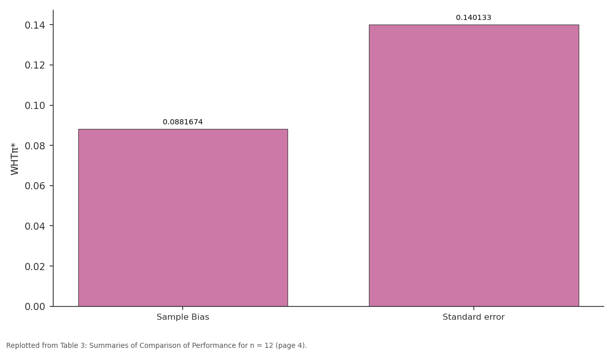
WHTπ*: Sample Bias vs Standard error
Replotted from Table 3 (page 4) of the original paper. Every bar is the paper's own table value.
View source evidence ↗Figures & tables
From the original paper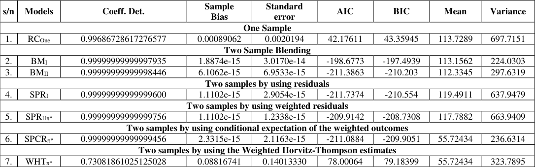 Table 3
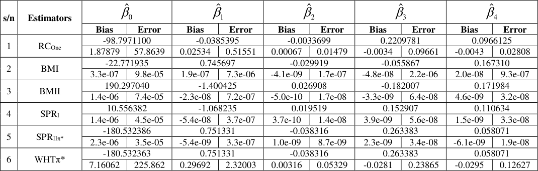 Table 4
Introduction
The enhanced relative efficacy of statistical analyses obtained by modeling and resolving measurement error using regression calibration by merging estimates from two samples is examined in this work. All statistical errors can be traced back to imperfections in measurement. This is referred to as "measurement error," and it occurs when one or more variables in an interest model cannot be measured consistently. Such errors can occur for a variety of reasons, the most common of which are sample and instrument faults.
Exposure variable measurement error
In a variety of study disciplines, measurement inaccuracy in exposure factors has been frequently shown. Measurement error is defined as the difference between a variable's true and measured values [8] . Memory bias can occur while doing historical studies that necessitate the researcher recalling and documenting earlier experiences. Biological variations and laboratory equipment faults can also create measurement errors in a study. Assessing exposure accuracy has long been an issue in research on exposures and health effects [7] . This study investigates the bias in exposure-outcome correlations that occurs when exposure variables are recorded incorrectly. Due to the various exposures and accompanying inaccuracies, the exposure-outcome connection may be skewed in any way [5] . The presence of measurement error in the exposure problem has sparked a wave of technique research, with the initial focus on understanding the effects of measurement error on the relationship between exposure and outcome and, more recently, on developing statistical approaches to correct for exposure measurement error [1, [3, 8, 4] .
The two sample approach for improving the efficiency of measurement error correction
In this study, two-sample approaches for enhancing measurement error regression and calibration accuracy were examined. Assume two distinct samples and gather pertinent information about the population as a whole. The study offered four approaches for integrating data from the two samples in order to provide a single set of more accurate estimates of a population number or population characteristic. In general, this issue has been solved by combining independent estimates from the two samples and weighting them by the reciprocal of their calculated variances [6] . The two data sets might alternatively be combined and the weights on each sampled unit adjusted proportionately [5] . The study also generated a variation of the Horvitz-Thompson estimate by taking the square root of the conditional expectation of the product of the estimates from the two samples based on the predictor variables of a regression function.
Objectives 2.1 General Objective
A comparison of two sample approaches to regression calibration for measurement error correction.
Specific Objective
Comparison of four approaches using coefficients of determination, small sample bias and standard error.
Design-based approaches 3.1 Blended Methodology I
The blended model for the study is a weighted regression of the conditional expectations of predictor variables, where the weights are the expected values of the outcomes from the two samples [9] :
Blended Methodology II
The blended model, which is the regression of the conditional expectancies of the predictor variables, was developed from the study, where the weights are the variance values of the outcomes from the two samples, and greater weight is given to the result with the lowest variance, as shown below [9] :
Model-assisted Semi-parametric regression
In this study, model-assisted semi-parametric regression was used to estimate non-parametric regression, which was adapted from [2]. [2] defines a model-assisted estimator as a design-unbiased estimator, as seen below [9] :
The Horvitz-Estimator
In our investigation, the Horvitz-Thompson estimator was used as a baseline to examine the performance of the novel models in terms of coefficient of determination, confidence intervals, sample bias, and standard error [9] .
Model-assisted Semi-parametric Conditional regression
In the study, the Horvitz-Thompson model was tweaked in the same way to develop models that outperformed it. It is the regression of the conditional expectation of the square root of the product of two weighted Horvitz-Thompson estimators [9] :
Strategies for combining the two samples
The table 1 below gives strategies used to combined estimates from the two, [9] [1.] Combining estimates from two samples by blended methodology using expected values of the outcomes Blended Methodology I, BMI ( ) ( )
v̂l= Larger variance, v̂s= Smaller variance
SPRI T E T x x x x = [4.] Combining estimates from two samples by using weighted residuals
Semiparametric regression II, SPRII
] Combining estimates from two samples by using conditional expectation of the weighted outcomes Semiparametric Conditional Regression, SPCR ( )
Finite small sample properties of estimators
The first attribute is concerned with the mean position of the estimator's distribution.
Biasedness -An estimator's bias is defined as var θ θ < (5.2)
Results
For each model plan, we ran the simulation 10,000 times. We used software programs built for statistical analysis in R. Table 3 shows that the Models have greater coefficients of determination, sample bias and sample standard error than the WHTπ*, and so are more efficient for real Data for n = 12. Where WHTπ* is our reference estimator, the Weighted Horvitz-Thompson Estimator. RCone is the regression calibration done using only one sample and it is evident from the coefficient of determination that ii falls short when compared to the other estimators while it out-performs WHTπ*.
| s/n | Models | Coeff. Det. | Sample Bias | Standard error | AIC | BIC | Mean | Variance |
|---|---|---|---|---|---|---|---|---|
| One Sample | ||||||||
| 1. | RCOne | 0.99686728617276577 | 0.00089062 | 0.0020194 | 42.17611 | 43.35945 | 113.7289 | 697.7151 |
| Two Sample Blending | ||||||||
| 2. | BMI | 0.99999999999997935 | 1.8874e-15 | 3.0170e-14 | -198.6773 | -197.4939 | 113.1562 | 224.0303 |
| 3. | BMII | 0.99999999999998446 | 6.1062e-15 | 6.9533e-15 | -211.3863 | -210.203 | 112.3345 | 297.6319 |
| Two samples by using residuals | ||||||||
| 4. | SPRI | 0.99999999999999600 | 1.1102e-15 | 2.9054e-15 | -211.7374 | -210.554 | 119.4911 | 637.9479 |
| Two samples by using weighted residuals | ||||||||
| 5. | SPRIIπ* | 0.99999999999999756 | 1.1102e-15 | 1.2338e-15 | -209.9142 | -208.7308 | 117.7882 | 663.9409 |
| Two samples by using conditional expectation of the weighted outcomes | ||||||||
| 6. | SPCRπ* | 0.99999999999999456 | 2.3315e-15 | 2.1163e-15 | -211.0884 | -209.9051 | 55.72434 | 236.6314 |
| Two samples by using the Weighted Horvitz-Thompson estimates | ||||||||
| 7. | WHTπ* | 0.73081861025125028 | 0.08816741 | 0.14013330 | 78.00064 | 79.18399 | 55.72434 | 323.7895 |
Table text extracted from the original PDF; superscript letters are shown inline. The original table image is below.
View original table image
Figures and tables from the paper
| s/n | Estimators | ˆ β 0 | — | βˆ 1 | — | ˆ β 2 | — | ˆ β 3 | — | ˆ β 4 | — |
|---|---|---|---|---|---|---|---|---|---|---|---|
| Bias | Error | Bias | Error | Bias | Error | Bias | Error | Bias | Error | ||
| 1 | RCOne | -98.7971100 | -0.0385395 | -0.0033699 | 0.2209781 | 0.0966125 | |||||
| 1.87879 | 57.8639 | 0.02534 | 0.51551 | 0.00067 | 0.01479 | -0.0034 | 0.09661 | -0.0043 | 0.02808 | ||
| 2 | BMI | -22.771935 | 0.745697 | -0.029919 | -0.055867 | 0.167310 | |||||
| 3.3e-07 | 9.8e-05 | 1.9e-07 | 7.3e-06 | -4.1e-09 | 1.7e-07 | -4.8e-08 | 2.2e-06 | 2.0e-08 | 9.3e-07 | ||
| 3 | BMII | 190.297040 | -1.400425 | 0.026908 | -0.182007 | 0.171984 | |||||
| 1.4e-06 | 7.4e-05 | -2.3e-08 | 7.2e-07 | -5.0e-10 | 1.7e-08 | -3.3e-09 | 6.4e-08 | 4.6e-09 | 3.2e-08 | ||
| 4 | SPRI | 10.556382 | -1.068235 | 0.019519 | 0.152907 | 0.110634 | |||||
| 1.4e-06 | 4.5e-05 | -5.4e-08 | 3.7e-07 | 3.7e-10 | 1.4e-08 | 3.9e-09 | 5.6e-08 | 1.5e-09 | 3.3e-08 | ||
| 5 | SPRIIπ* | -180.532386 | 0.751331 | -0.038316 | 0.263383 | 0.058071 | |||||
| 2.3e-06 | 3.5e-05 | -5.4e-09 | 3.3e-07 | 1.0e-09 | 8.7e-09 | 2.3e-09 | 3.4e-08 | -6.1e-09 | 1.9e-08 | ||
| 6 | WHTπ* | -180.532363 | 0.751331 | -0.038316 | 0.263383 | 0.058071 | |||||
| 7.16062 | 225.862 | 0.29692 | 2.32003 | 0.00316 | 0.05329 | -0.0281 | 0.23865 | -0.0295 | 0.12627 |
Table text extracted from the original PDF; superscript letters are shown inline. The original table image is below.
View original table image
References
6 in the original paper- Agogo GO. van der Voet H, van 't Veer P, Ferrari P, et al. Use of Two-Part Regression Calibration Model to Correct for Measurement Error in Episodically Consumed Foods in a Single-Replicate Study Design: EPIC Case Study. PLoS ONE. 2014;9(11):1-15. DOI: 10.1371/journal.pone.0113160.
- Breidt FJ, Opsomer JD. Local polynomial regression estimators in survey sampling, Annals of Statistics. 2000;28(4):1026-1053.
- Dorfman AH. The two sample problem, Proceedings of the Joint Statistical Meetings, Section of Survey Research Methods. Journal of the American Statistical Association. 2008;87:998-1004.
- Merkouris T, Combining independent regression estimators from multiple surveys. Journal of the American Statistical Association. 2004;99(468):11311139.
- Thomas D, Stram D, Dwyer J. Exposure Measurement Error: Influence on Exposure-Disease relationships and Methods of correction. Annual Review of Public Health. 1993;14(1):69-93.
- Kamun SJ, Nyakundi C, Simwa R. Two Sample Approaches to Regression Calibration for Measurement Error Correction. International Journal of Statistical Distributions and Applications. 1993, 2023;9(1):35-40.